Structure Factor
The multi-scale statistical behavior of a polymer chain is frequently characterized by the single-chain structure factor. The structure factor is directly measured in a scattering experiment, and correlating scattering experiments with theoretical models provides insight into the physical behavior in polymeric fluids. From a theoretical perspective, the single-chain structure factor acts as an input for treating many-chain systems including concentration fluctuations. Although the structure factors for both a flexible Gaussian chain and a rigid rod are easily expressible, the structure factor of a semiflexible polymer is considerably more difficult to predict theoretically, largely due to the challenges in acquiring analytical expressions for the governing chain statistics. Our goal in this section is to apply our exact results to predict the structure factor for the wormlike chain model that is valid over the entire range of scattering vectors and chain lengths.
Two-point Structure Factor
We define the structure factor to be
where \(\vec{k}\) is the scattering vector, and the angular brackets denote an average with respect to the specific model that governs the chain statistics. Our current manuscript contains exact results that permit the evaluation of the structure factor for the wormlike chain model without excluded volume interactions. Our definition for the structure factor differs from the conventional definition by an extra factor of \(1/L\), thus rendering a dimensionless structure factor that tends to one at zero scattering vector.
For the wormlike chain model, the structure factor is given by
where \(K = 2 l_{p} | \vec{k} |\), \(\mathcal{L}^{-1}\) implies a Laplace inversion from \(p\) to \(N=L/(2l_{p})\), and \(G(K;p)\) is the wormlike chain Green function. The structure factor is expressible in terms of the magnitude of the scattering vector due to the rotational invariance of the governing statistics. Using results given in Wormlike Chain Green’s Function, we write the structure factor as
where \(j_{0}^{(+)}(K;p)\) and \(\partial_{p} j_{0}^{(+)}(K;p)\) are continued-fraction functions that are defined in Wormlike Chain Green’s Function. Equation (1) is evaluated using methods outlined in Wormlike Chain Green’s Function. to find the eigenvalues \(\mathcal{E}_{l}\) and to calculate \(j_{0}^{(+)}\) and \(\partial_{p} j_{0}^{(+)}\). The structure factor given by Eq. (1) is expressed in arbitrary number of dimensions \(D\), which is generally useful for treating many-chain systems.
In Ref. [Spakowitz2004], we present realizations of the structure factor for the wormlike chain model in 3 dimensions, demonstrating that our exact results for wormlike chain statistics in 3 dimensions capture the structure factor over all chain lengths and scattering vectors. Equation (1), along with the techniques provided in Wormlike Chain Green’s Function, provide a convenient methodology for calculating the structure factor as a comparison with scattering experiments. Specifically, the infinite summation in Eq. (1) is truncated at a finite cutoff, and the partial summation is evaluated using methods to evaluate \(\mathcal{E}_{l}\) found in Wormlike Chain Green’s Function. For most calculations, only a couple of terms are necessary to achieve accurate realizations of the structure factor. For example, the structure factor in 3 dimensions for a chain of length \(N=0.1\) requires only 4 terms in the summation to achieve accuracy within 1.76 percent difference from a more accurate calculation with 30 terms in the summation (emph{i.e.} completely converged in its numerical behavior). Since the terms in the summation decay exponentially with \(N\), larger \(N\) values require fewer terms. To illustrate this, we note that the structure factor in 3 dimensions for a slightly larger chain of length \(N=0.5\) calculated with 4 terms in the summation is within \(1.05 \times 10^{-4}\) percent difference from the calculation with 30 terms in the summation. Therefore, most practical applications of Eq. (1) require the inclusion of only a couple of terms in the summation.
Three-point and Four-point Density Correlation Functions
We now extend the definition of the structure factor to include 3-point and 4-point correlation functions, as these serve as necessary input for a density expansion of the free energy under the random phase approximation (RPA) to a field-theoretic treatment of polymer solutions. The structure factors form the basis of the cubic and quartic vertex functions in the free energy expansion due to the connection between the structure factor and correlated density fluctuations in the solution. We discuss the evaluation of these functions below.
Three-point structure factor
We define the 3-point structure factor \(S^{(3)}(\vec{k}_{1}, \vec{k}_{2})\) as
We note that the 3-point density corelations depend on 3 k-vectors, which satisfy \(\vec{k}_{1}+\vec{k}_{2}+\vec{k}_{3}=0\) or \(\vec{k}_{3} = -\vec{k}_{1}-\vec{k}_{2}\). For the wormlike chain model, we leverage the Green’s function to evaluate this average. The 3-point structure factor is written in terms of the Green’s function to be
where \(\vec{K}_{i} = 2 l_{p} \vec{k}_{i}\). In this calculation, we need to evaluate the rotated spherical harmonics (see Rotation of spherical harmonics).
Four-point structure factor
We define the 4-point structure factor \(S^{(4)}(\vec{k}_{1}, \vec{k}_{2})\) as
We note that the 4-point density corelations depend on 4 k-vectors, which satisfy \(\vec{k}_{1}+\vec{k}_{2}+\vec{k}_{3}+\vec{k}_{4}=0\) or \(\vec{k}_{4} = -\vec{k}_{1}-\vec{k}_{2}-\vec{k}_{3}\). For the wormlike chain model, we leverage the Green’s function to evaluate this average. The 4-point structure factor is written in terms of the Green’s function to be
where the summation over \(\gamma\) cycles through the 12 variants that account for all distinct time orderings of the integrals. The
\(\gamma\) |
integral ordering |
\(\vec{K}_{a}^{(\gamma)}\) |
\(\vec{K}_{b}^{(\gamma)}\) |
\(\vec{K}_{c}^{(\gamma)}\) |
|---|---|---|---|---|
1 |
\(s_{4}>s_{3}>s_{2}>s_{1}\) |
\(\vec{K}_{1}+\vec{K}_{2}+\vec{K}_{3}\) |
\(\vec{K}_{1}+\vec{K}_{2}\) |
\(\vec{K}_{1}\) |
2 |
\(s_{4}>s_{3}>s_{1}>s_{2}\) |
\(\vec{K}_{1}+\vec{K}_{2}+\vec{K}_{3}\) |
\(\vec{K}_{1}+\vec{K}_{2}\) |
\(\vec{K}_{2}\) |
3 |
\(s_{4}>s_{2}>s_{3}>s_{1}\) |
\(\vec{K}_{1}+\vec{K}_{2}+\vec{K}_{3}\) |
\(\vec{K}_{1}+\vec{K}_{3}\) |
\(\vec{K}_{1}\) |
4 |
\(s_{4}>s_{1}>s_{3}>s_{2}\) |
\(\vec{K}_{1}+\vec{K}_{2}+\vec{K}_{3}\) |
\(\vec{K}_{2}+\vec{K}_{3}\) |
\(\vec{K}_{2}\) |
5 |
\(s_{4}>s_{2}>s_{1}>s_{3}\) |
\(\vec{K}_{1}+\vec{K}_{2}+\vec{K}_{3}\) |
\(\vec{K}_{1}+\vec{K}_{3}\) |
\(\vec{K}_{3}\) |
6 |
\(s_{4}>s_{1}>s_{2}>s_{3}\) |
\(\vec{K}_{1}+\vec{K}_{2}+\vec{K}_{3}\) |
\(\vec{K}_{2}+\vec{K}_{3}\) |
\(\vec{K}_{3}\) |
7 |
\(s_{3}>s_{4}>s_{2}>s_{1}\) |
\(-\vec{K}_{3}\) |
\(\vec{K}_{1}+\vec{K}_{2}\) |
\(\vec{K}_{1}\) |
8 |
\(s_{3}>s_{4}>s_{1}>s_{2}\) |
\(-\vec{K}_{3}\) |
\(\vec{K}_{1}+\vec{K}_{2}\) |
\(\vec{K}_{2}\) |
9 |
\(s_{2}>s_{4}>s_{3}>s_{1}\) |
\(-\vec{K}_{2}\) |
\(\vec{K}_{1}+\vec{K}_{3}\) |
\(\vec{K}_{1}\) |
10 |
\(s_{1}>s_{4}>s_{3}>s_{2}\) |
\(-\vec{K}_{1}\) |
\(\vec{K}_{2}+\vec{K}_{3}\) |
\(\vec{K}_{2}\) |
11 |
\(s_{2}>s_{4}>s_{1}>s_{3}\) |
\(-\vec{K}_{2}\) |
\(\vec{K}_{1}+\vec{K}_{3}\) |
\(\vec{K}_{3}\) |
12 |
\(s_{1}>s_{4}>s_{2}>s_{3}\) |
\(-\vec{K}_{1}\) |
\(\vec{K}_{2}+\vec{K}_{3}\) |
\(\vec{K}_{3}\) |
Functions contained with the ‘wlcstruc’ module
-
wlcstat.wlcstruc.calc_int_mag(length_kuhn, poles_vec, frac_zero=1.0)[source]¶ Evaluate the magnitude of the integral for a list of poles (including repeats). This algorithm includes cases for single, double, and triple poles (as needed in evaluation of correlation functions)
- Parameters
length_kuhn (float) – The length of the chain in Kuhn lengths
poles_vec (float (array)) – Array of poles
frac_zero (float) – Multiplicative factor for contributions from poles at p=0
- Returns
int_mag – Value of the integral over chain length for the five poles
- Return type
float
-
wlcstat.wlcstruc.calc_s4_int_mag(length_kuhn, pole1, pole2, pole3, frac_zero=1.0)[source]¶ Evaluate the magnitude of the integral for a list of poles (including repeats). This algorithm includes cases for single, double, and triple poles (as needed in evaluation of correlation functions)
- Parameters
length_kuhn (float) – The length of the chain in Kuhn lengths
poles_vec (float (array)) – Array of poles
frac_zero (float) – Multiplicative factor for contributions from poles at p=0
- Returns
int_mag – Value of the integral over chain length for the five poles
- Return type
float
-
wlcstat.wlcstruc.eval_legendre(rho, mu=0, alpha_max=25)[source]¶ Evaluate the vector of Legendre polynomial values
- Parameters
rho (float) – Cos theta of the angle
mu (int) – Value of the z-momentum quantum number
alpha_max (int) – Maximum number of polynomials evaluated (default 25)
- Returns
legendre_poly – Vector of Legendre polynomials
- Return type
float
-
wlcstat.wlcstruc.s2_wlc(k_val_vector, length_kuhn, dimensions=3, alpha_max=25)[source]¶ s2_wlc - Evaluate the 2-point structure factor for the wormlike chain model
- Parameters
k_val_vector (float (array)) – The value of the Fourier vector magnitude \(K\)
length_kuhn (float (array)) – The length of the chain in Kuhn lengths
dimensions (int) – The number of dimensions (default to 3 dimensions)
alpha_max (int) – Maximum number of poles evaluated (default 25)
- Returns
s2 – Structure factor for the wormlike chain model for every k_val in k_val_vector
- Return type
float (vector)
Notes
See Mehraeen, et al, Phys. Rev. E, 77, 061803 (2008). (Ref [Mehraeen2008])
-
wlcstat.wlcstruc.s3_wlc(k1_val_vector, k2_val_vector, length_kuhn, dimensions=3, alpha_max=15)[source]¶ s3_wlc - Evaluate the 3-point structure factor for the wormlike chain model
- Parameters
k1_val_vector (float (array)) – The value of the Fourier vector \(\vec{K}_{1}\)
k2_val_vector (float (array)) – The value of the Fourier vector \(\vec{K}_{2}\)
length_kuhn (float (array)) – The length of the chain in Kuhn lengths
dimensions (int) – The number of dimensions (default to 3 dimensions)
alpha_max (int) – Maximum number of poles evaluated (default 25)
- Returns
s3_wlc – 3-point Structure factor for the wormlike chain model for every k1_val and k2_val in k1_val_vector and k2_val_vector
- Return type
float (vector)
Notes
See Mehraeen, et al, Phys. Rev. E, 77, 061803 (2008). (Ref [Mehraeen2008])
-
wlcstat.wlcstruc.s4_wlc(k1_val_vector, k2_val_vector, k3_val_vector, length_kuhn, dimensions=3, alpha_max=10)[source]¶ s4_wlc - Evaluate the 4-point structure factor for the wormlike chain model
- Parameters
k1_val_vector (float (array)) – The value of the Fourier vector \(\vec{K}_{1}\)
k2_val_vector (float (array)) – The value of the Fourier vector \(\vec{K}_{2}\)
k3_val_vector (float (array)) – The value of the Fourier vector \(\vec{K}_{2}\)
length_kuhn (float (array)) – The length of the chain in Kuhn lengths
dimensions (int) – The number of dimensions (default to 3 dimensions)
alpha_max (int) – Maximum number of poles evaluated (default 25)
- Returns
s4_wlc – 4-point Structure factor for the wormlike chain model for every k1_val, k2_val, k3_val in k1_val_vector, k2_val_vector, k3_val_vector
- Return type
float (vector)
Notes
See Mehraeen, et al, Phys. Rev. E, 77, 061803 (2008). (Ref [Mehraeen2008])
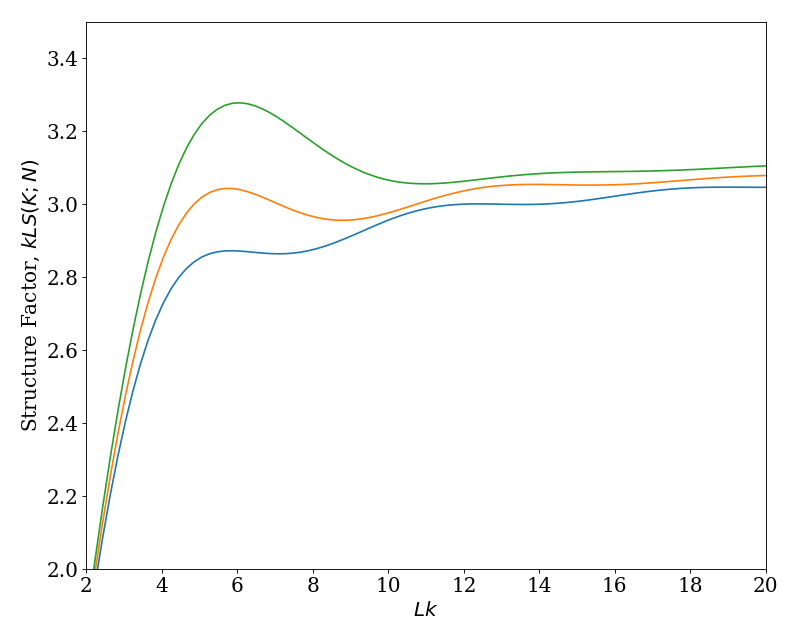
Example usage of ‘s2_wlc’
This plot shows the structure factor for the wormlike chain in 3 dimensions over a range of \(K\) for \(N = 0.1\), \(0.5\), and \(1.0\). This plot is a reproduction of Fig. 2 in Ref. [Spakowitz2004].
(Source code, png, hires.png, pdf)
