Wormlike Chain Green’s Function

We consider the end-to-end distribution function \(G(\vec{R},\vec{u}|\vec{u}_{0};L)\) (or Green’s function), which gives the probability that a chain that begins at the origin with initial orientation \(\vec{u}_{0}\) will have end position \(\vec{R}\) and final orientation \(\vec{u}\). The Green’s function \(G(\vec{R},\vec{u}|\vec{u}_{0};L)\) is written as

\[G(\vec{R},\vec{u}|\vec{u}_{0};L) = \int_{\vec{u}(s=0)=\vec{u}_{0}}^{\vec{u}(s=L)=\vec{u}} \hspace{-0.3in} \mathcal{D}[\vec{u}(s)] \exp \left\{ -\beta \mathcal{H}_{0} [\vec{u}(s)] \right\} \delta \left( \vec{R}-\int_{0}^{L}ds \vec{u} \right),\]

where \(\delta\) is a Dirac delta function that restricts the path integration to those paths that satisfy the fixed end separation \(\vec{R}\). The path integral formulation of the Green function is used to find the governing “Schrödinger” equation [Yamakawa1997]

\[\left( \frac{\partial}{\partial L} - \frac{1}{2l_{p}} \tilde{\nabla}^{2}_{D} + \vec{u} \cdot \vec{\nabla}_{R} \right) G(\vec{R},\vec{u}|\vec{u}_{0};L)= \delta \left( L \right) \delta ( \vec{R} ) \delta \left( \vec{u} - \vec{u}_{0} \right),\]

where \(\tilde{\nabla}^{2}_{D}\) is the \(D\)-dimensional angular Laplacian, and \(\vec{\nabla}_{R}\) is the \(D\)-dimensional gradient operator.

Upon \(D\)-dimensional Fourier transforming from the variable \(\vec{R}\) to the wavevector \(\vec{k}\), our problem becomes that of a single wormlike chain with Hamiltonian

\[\beta \mathcal{H} = \beta \mathcal{H}_{0} + \beta \mathcal{H}_{ext} = \frac{l_{p}}{2} \int_{0}^{L} ds \left( \frac{\partial \vec{u}}{\partial s} \right)^{\! \! 2} -i\vec{k} \cdot \int_{0}^{L}ds \vec{u}.\]

The external Hamiltonian \(\beta \mathcal{H}_{ext}\) naturally emerges in the Fourier transform of the end-to-end distribution function \(G(\vec{R},\vec{u}|\vec{u}_{0};L)\) due to the end-position constraint. The corresponding “Schrödinger” equation in Fourier space is

\[\left( \frac{\partial}{\partial L} - \frac{1}{2l_{p}} \tilde{\nabla}^{2}_{D} - i \vec{k}\cdot \vec{u} \right) G(\vec{k},\vec{u}|\vec{u}_{0};L)= \delta \left( L \right) \delta \left( \vec{u} - \vec{u}_{0} \right),\]

which demonstrates the direct correspondence between our problem and that of a rigid rotor in a dipole field.

Exact results for the Green’s function are provided in Refs. [Spakowitz2004], [Spakowitz2005], [Spakowitz2006], and [Mehraeen2008], which give solutions with and without end constraints and in arbitrary dimensions \(D\). For example, the solution to the orientation-independent Green function in Fourier-Laplace space (i.e. Fourier transformed from \(\vec{R}\) to \(\vec{k}\) and Laplace transformed from \(N\) to \(p\))

(1)\[G(\vec{K};p) = \frac{1}{P_{0}+\frac{\left(a_{1} K\right)^2}{P_{1}+ \frac{\left(a_{2} K\right)^2}{P_{2}+\frac{\left(a_{3} K\right)^2}{\cdots}}}},\]

where \(\vec{K}=2l_{p} \vec{k}\), \(K\) is the magnitude of \(\vec{K}\), \(P_{\lambda}=p+ \lambda (\lambda+D-2)\), and \(a_{\lambda} = \left[\frac{\lambda (\lambda+D-3)}{(2\lambda+D-2)(2\lambda+D-4)}\right]^{1/2}\). A detailed derivation of this \(D\)-dimensional solution is found in Ref. [Mehraeen2008]. We note that this exact solution produces identical results as those given in Ref. [Spakowitz2004] for 2- and 3-dimensional solutions.

Methods to Evaluate the Wormlike Chain Green’s Function

The Green’s function (e.g. (1)) is written in Fourier-Laplace space. Thus, evaluation of the Green’s function requires inversion to real space \(\vec{R}\) and \(N\). The python module ‘wlcgreen’ contains python code to numerically invert the Fourier and Laplace transforms to render real-space solutions. The procedure followed in this module is as follows:

• Laplace-space inversion (from \(p\) to \(N\)): Numerical Laplace inversion using residue theorem based on evaluation of the singularities in \(G\)

• Fourier-space inversion (from \(\vec{k}\) to \(\vec{R}\)): Numerical Fourier inversion by numerical integration over \(\vec{k}\)

These steps are performed sequentially, such that Laplace inversion is first followed by Fourier inversion. The Spakowitz lab has utilized other numerical approaches for these steps. For example, numerical Laplace inversion can also be performed by numerical complex integration of the Bromwich integral, but this approach is not integrated into the ‘wlcgreen’ module.

The orientation-independent Green’s function \(G(\vec{K};p)\) in (1) serves as a useful example for our numerical procedures. Below, we discuss the two steps for the real-space inversion for this function.

Step 1: Laplace-space inversion

The Laplace-space inversion requires us to determine the poles \(\mathcal{E}_{\alpha}\) (all simple and generally complex). Mathematically, this is written as

\[j (K; p = \mathcal{E}_{\alpha}) = \frac{1}{G(K; p = \mathcal{E}_{\alpha})} = 0\]

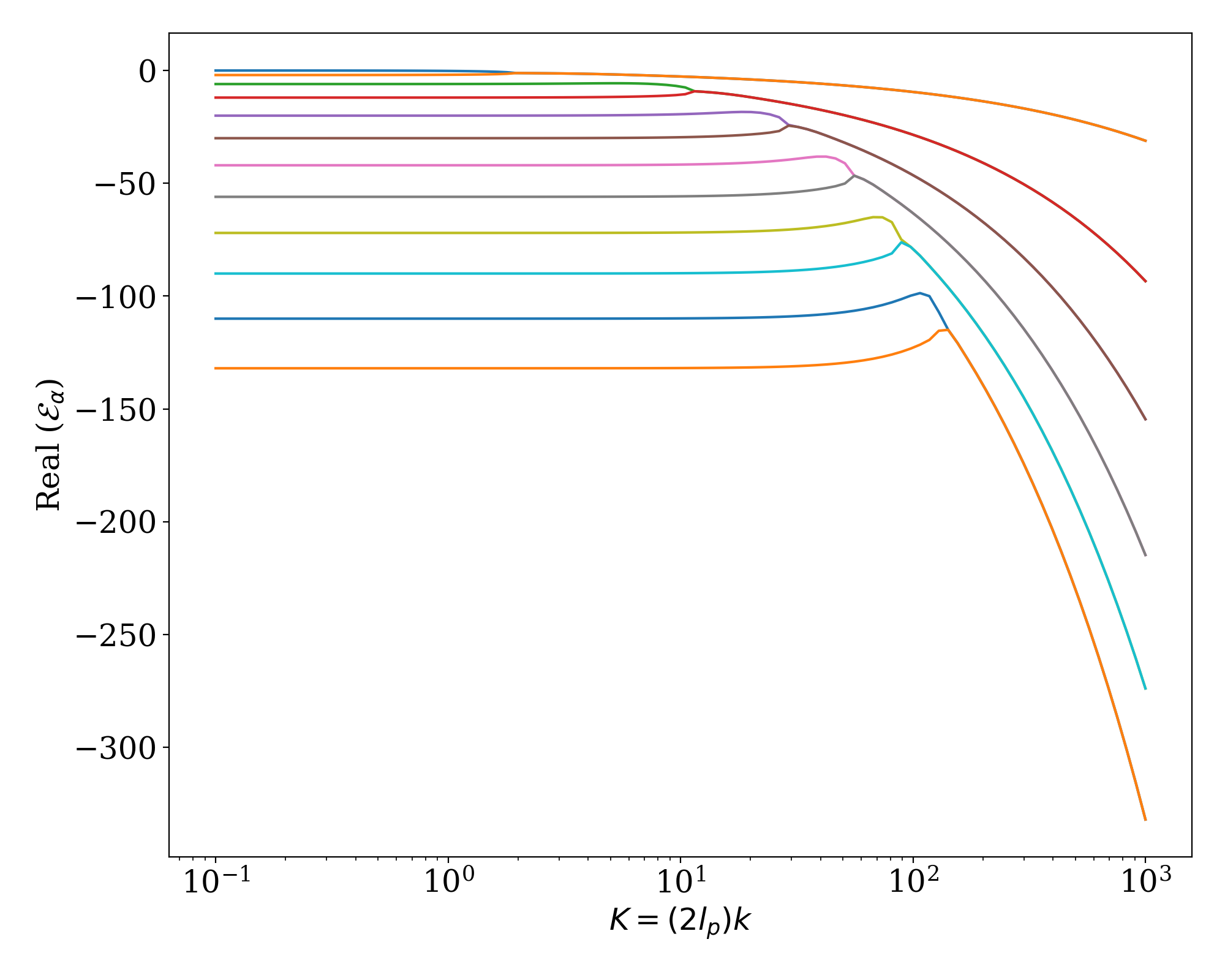
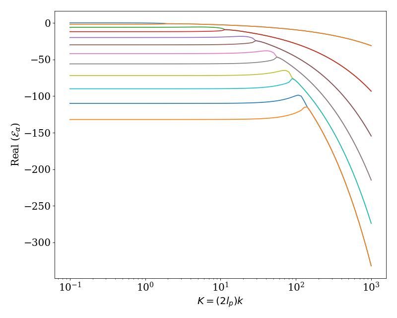
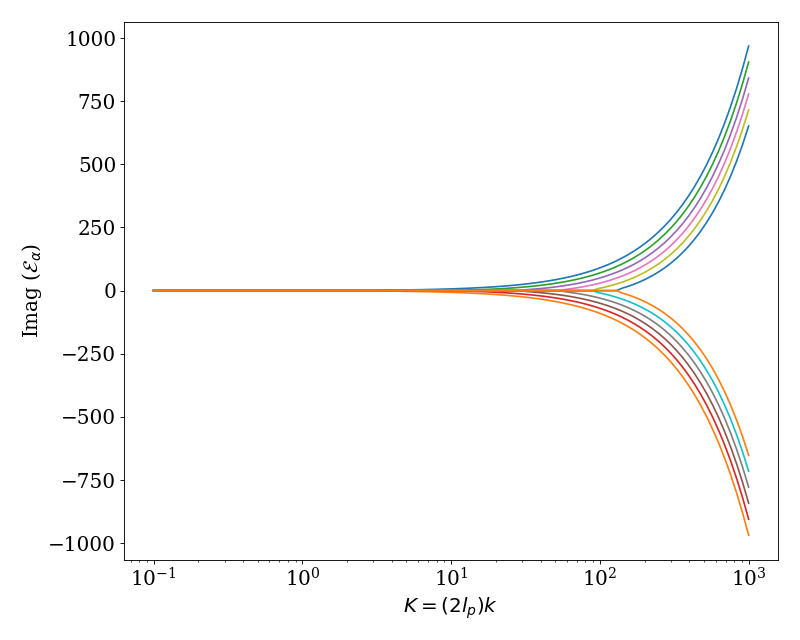
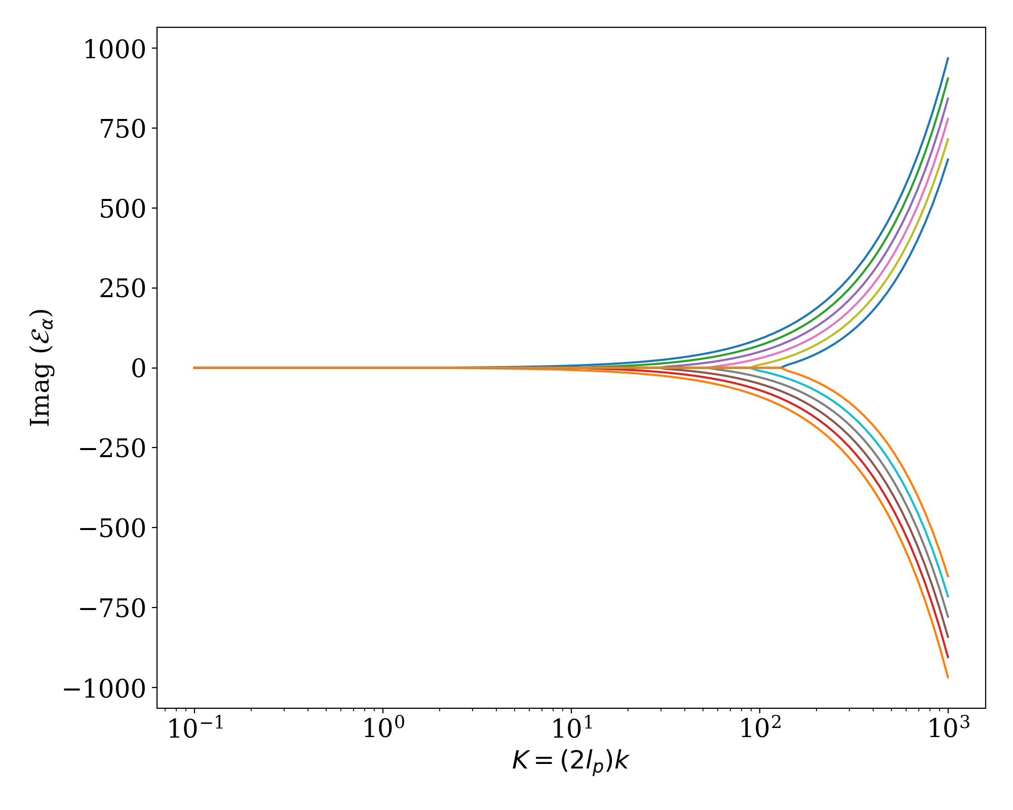
for \(\alpha = 0, 1, \ldots\) gives the infinite set of poles within the infinite continued fraction. In practice, the real part of \(\mathcal{E}_{\alpha}\) becomes increasingly negative with increasing \(\alpha\), and a cutoff \(\alpha = \alpha_{\mathrm{max}}\) is invoked for any given \(N\). We note that \(\mathcal{E}_{\alpha} \rightarrow -\alpha (\alpha+D-2)\) (unperturbed eigenvalues of the hyperspherical harmonics) as \(K \rightarrow 0\) and becomes more negative with increasing \(K\) (see Ref [Mehraeen2008]). We determine \(\alpha_{\mathrm{max}}\) based on the \(K=0\) magnitude of \(G\) for a given \(N\).

The Laplace inversion is then determined by evaluating the residues in the complex plane. The is written as

\[G (K; N) = \sum_{\alpha = 0}^{\alpha_{\mathrm{max}}} \mathop{\mathrm{Res}}_{p = \mathcal{E}_{\alpha}} \left[ G(K; p) \exp \left( p N \right) \right] = \sum_{\alpha = 0}^{\alpha_{\mathrm{max}}} \lim_{p \rightarrow \mathcal{E}_{\alpha}} \left[ ( p - \mathcal{E}_{\alpha}) G(K; p) \exp \left( p N \right) \right] = \sum_{\alpha = 0}^{\alpha_{\mathrm{max}}} \frac{1}{\partial_{p} j (K; p = \mathcal{E}_{\alpha})} \exp \left( \mathcal{E}_{\alpha} N \right)\]

The final form arises from the fact that all of the poles \(\mathcal{E}_{\alpha}\) are simple. From this development, the Laplace inversion requires evaluation of two quantities: \(\mathcal{E}_{\alpha}\) (for \(\alpha = 0, 1, \ldots, \alpha_{\mathrm{max}}\)) and \(\partial_{p} j (K; p = \mathcal{E}_{\alpha}) = \frac{\partial j (K; p = \mathcal{E}_{\alpha})}{\partial p}\). We leverage several numerical and asymptotic methods to find the poles \(\mathcal{E}_{\alpha}\) (see [Mehraeen2008] for a detailed description of these methods).

This basic approach is extended to Green’s function evaluation with fixed end orientation (i.e. the orientation-dependent Green’s function). Turning back to the general Green’s function (i.e. including end orientations), we have

\[G(\vec{K},\vec{u}|\vec{u}_{0};p) = \frac{1}{\Omega_{D}} \sum_{\lambda} \sum_{\lambda_{0}} \sum_{\mathbf{\mu}} Y^{(D)}_{\lambda;\mathbf{\mu}} (\vec{u}') Y^{(D)*}_{\lambda_{0};\mathbf{\mu}}(\vec{u}_{0}') \mathcal{G}_{\lambda,\lambda_{0}}^{\mu}(K;p).\]

This spherical harmonic expansion requires evaluation of the Laplace inverse of \(\mathcal{G}_{\lambda,\lambda_{0}}^{\mu_{1}}(K;p)\) (i.e. spherical-harmonic transform of the Green’s function). The evaluation of poles and residues of \(\mathcal{G}_{\lambda,\lambda_{0}}^{\mu}(K;p)\) utilizes similar approaches as outlined above and discussed in detail in Ref. [Mehraeen2008]. The primary difference is whether the residues and poles require evaluation for non-zero values of \(\mu\) and the residue evaluation must account for different \(\lambda\) and \(\lambda_{0}\). Poles and residues are evaluated for the additional index \(\mu\), which defines the \(z\)-component of the angular momentum (noting the Quantum Mechanical analogy of our problem). Inclusion of \(\mu\) requires definition of the cutoff \(\mu = \mu_{\mathrm{max}}\) that restricts the otherwise infinite summations within the inversion. Evaluation of the residues for all possible values of \(\lambda\) and \(\lambda_{0}\) (with a cutoff \(\lambda_{\mathrm{max}}\)) results in a residue matrix defined by \([\partial_{p} j_{\lambda,\lambda_{0}}^{\mu} (K;p = \mathcal{E}_{\alpha}^{\mu} ) ]^{-1}\), which is a \((\lambda_{\mathrm{max}} - \mu + 1) \times (\lambda_{\mathrm{max}} - \mu + 1)\) tensor for a given \(\mu\) and \(\mathcal{E}_{\alpha}^{\mu}\).

The following table shows the cases of whether non-zero values of \(\mu\) and \(\lambda\) need to be evaluated for the Laplace-inversion. We define the boolean parameters ‘mu_zero_only’ and ‘lam_zero_only’ to determine the family of residues and poles that need to be determined for a given Green’s function evaluation.

	\(G(K;N)\)	\(G(K,\vec{u}_{0};N)\)	\(G(K,\vec{u}|\vec{u}_{0};N)\)
‘mu_zero_only’	True	True	False
‘lam_zero_only’	True	False	False

We define a data structure that facilitates evaluation of the Laplace inversion but also enables the ‘wlcgreen’ module to dynamically grow the data structure, so residues and poles do not require re-evaluation if already evaluated at a given \(K\). We define the ‘green_properties’ library as follows

green_properties = { k_val1:[mu_zero_only, lam_zero_only, poles, residues],
                     k_val2:[mu_zero_only, lam_zero_only, poles, residues], ... }

For a given key in the library ‘k_val’, the elements are as follows

• ‘mu_zero_only’ is a boolean (True or False) that determines whether the poles and residues are evaluated for non-zero values of \(\mu\)

• ‘lam_zero_only’ is a boolean (True or False) that determines whether the residues are evaluated for non-zero \(\lambda\)

• ‘poles’ is an array of poles [size \((\alpha_{\mathrm{max}} + 1) \times (\mu_{\mathrm{max}} + 1)\)], which accounts for the value of ‘mu_zero_only’

• ‘residues’ is an array of residues [size \((\alpha_{\mathrm{max}} + 1) \times (\mu_{\mathrm{max}} + 1)\)] (to be discussed further)

Step 2: Fourier-space inversion

The Fourier inversion is found by numerically performing the integral

\[\begin{split}G(\vec{R};N) & = & \frac{1}{(2\pi)^{D}} \int d\vec{k} \exp \left( -i \vec{k} \cdot \vec{R} \right) G(K;N) \nonumber \\ & = & \frac{1}{(2 l_{p})^{D}} \frac{1}{(2 \pi)^{D/2}} \int_{0}^{\infty} d K K^{D-1} \frac{J_{D/2-1}(NrK)}{\left(NrK\right)^{D/2-1}} G(K;N)\end{split}\]

where \(\vec{K} = 2 l_{p} \vec{k}\) (\(K = |\vec{K}|\)), \(\vec{r} = \vec{R}/L\) (\(r = |\vec{r}|\)), and \(J_{n}(z)\) is the Bessel function of the first kind.

Integration over \(K\) is performed numerically from \(K=0\) to \(K=K_{\mathrm{cutoff}}\), where \(K_{\mathrm{cutoff}}\) is a cutoff value that is sufficiently large to achieve convergence. The \(K\)-step size in the numerical integration is chosen such that it satisfies a global accuracy threshold. In our calculation, we use a tolerance of \(10^{-20}\), which leads to an overall accuracy of \(10^{-15}\) for the real-space Green function.

Functions contained with the ‘wlcgreen’ module

wlcstat.wlcgreen.eval_poles_and_residues(k_val, mu, lam_zero_only=True, dimensions=3)

eval_poles_and_residues - Evaluate the poles and the residues for a given value of the Fourier vector magnitude \(K\)

Parameters

• k_val (float) – The value of the Fourier vector magnitude \(K\)

• mu (int) – Value of the mu parameter (\(z\)-component of the angular momentum)

• lam_zero_only (boolean) – Determines whether residues are determined for non_zero \(\lambda\) (default True)

• dimensions (int) – The number of dimensions (default to 3 dimensions)

Returns

• poles (complex float) – Evaluated poles for the given \(K\) and \(\mu\)

• residues (complex float) – Evaluated residues for the given \(K\) and \(\mu\)

Notes

See Mehraeen, et al, Phys. Rev. E, 77, 061803 (2008). (Ref [Mehraeen2008])

wlcstat.wlcgreen.gwlc_r(r_val, length_kuhn, dimensions=3, alpha_max=25, k_val_max=100000.0, delta_k_val_max=0.1)

gwlc_r - Evaluate the orientation-independent Green’s function for the wormlike chain model

Parameters

• r_val (float (array)) – The values of the end-to-end distance \(r = R/L\) to be evaluated

• length_kuhn (float (array)) – The length of the chain in Kuhn lengths

• dimensions (int) – The number of dimensions (default to 3 dimensions)

• alpha_max (int) – Maximum number of poles evaluated (default 25)

• k_val_max (float) – Cutoff value of \(K\) for numerical integration

• delta_k_val_max (float) – Maximum value of the integration step size

Returns

gwlc – The orientation-independent Green’s function [size len(r_val) x len(length_kuhn)]

Return type

float

Notes

See Mehraeen, et al, Phys. Rev. E, 77, 061803 (2008). (Ref [Mehraeen2008])

Example usage of ‘eval_poles_and_residues’

This plot shows the poles for the wormlike chain in 3 dimensions over a range of \(K\). This plot is a reproduction of Fig. 1 in Ref. [Mehraeen2008].

(Source code, png, hires.png, pdf)

(Source code, png, hires.png, pdf)

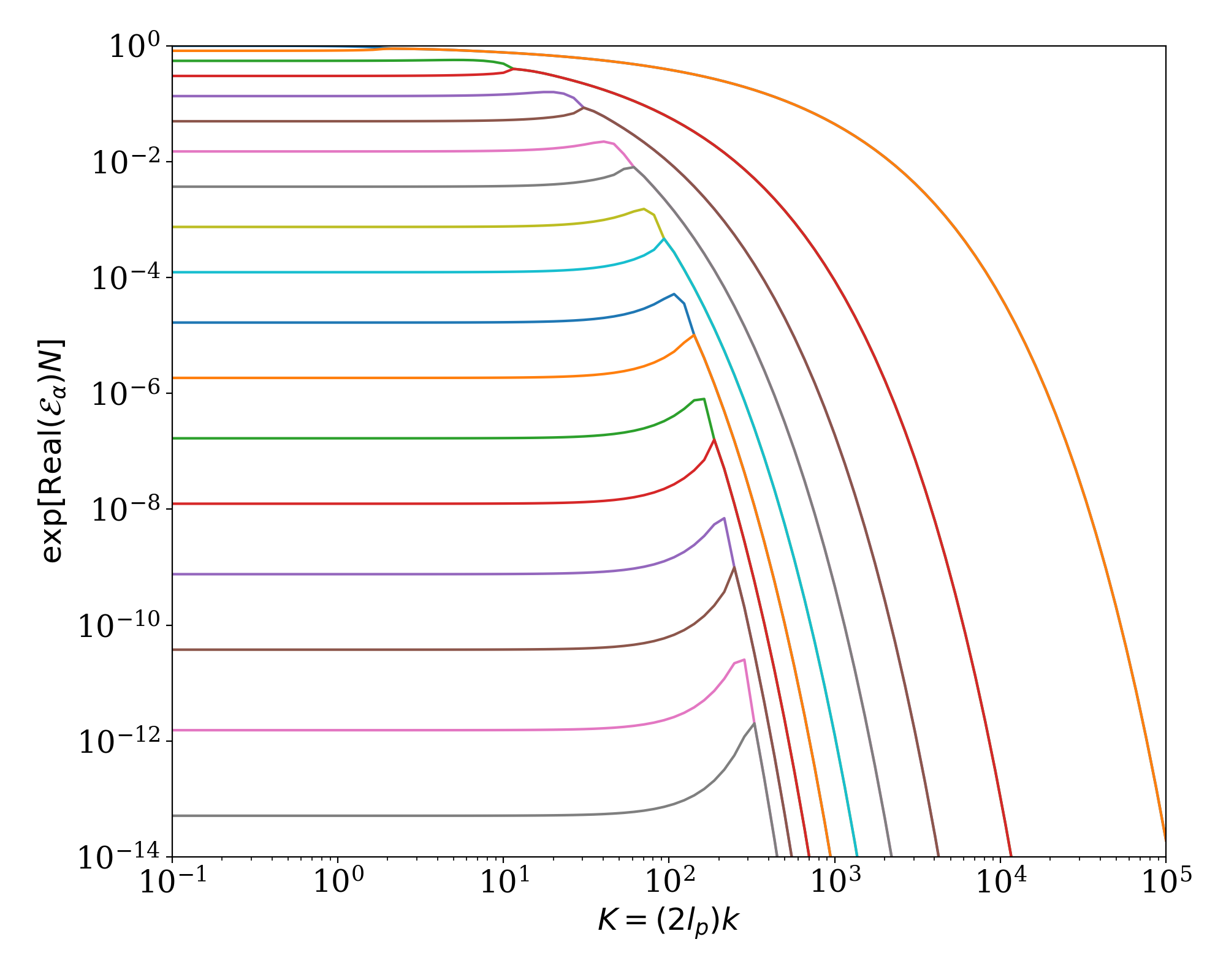
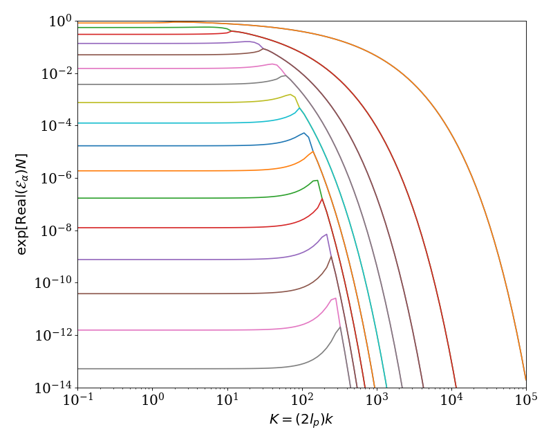
Another way to look at the poles is to consider the weight of the individual poles on the Fourier inversion. We consider a chain length \(N=0.1\), which is quite rigid. This plot shows the weight \(\exp \left[ \mathrm{Real} (\mathcal{E}_{\alpha} ) N \right)\) over a range of \(K\). We note that the \(y\)-scale in this plot is roughly coincident with machine precision \(10^{-14}\), so the \(k\)-range and the number of poles are the complete set necessary for Laplace inversion to machine precision accuracy for this chain length.

(Source code, png, hires.png, pdf)

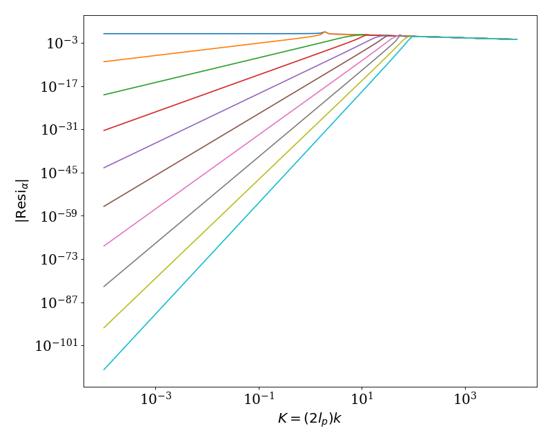
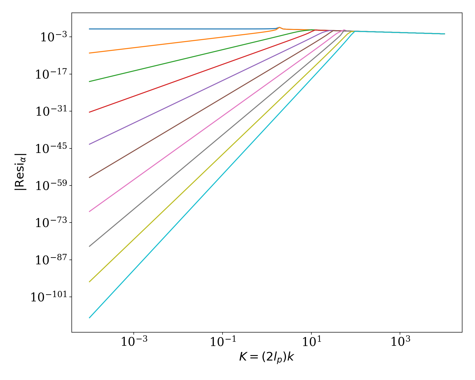
We now demonstrate the evaluation of the residues for \(\lambda = \lambda_{0} = 0\) and \(\mu = 0\) We show the residues values for the first 10 eigenvalues \(\mathcal{E}_{\alpha}\). Our numerical procedure utilizes the small-\(k\) and intermediate-\(k\) algorithms given in Ref. [Mehraeen2008], with a cross-over frequency of \(K_{\mathrm{cutoff}} = 0.01\).

(Source code, png, hires.png, pdf)