Average Quantities

The orientation Green function can be used to evaluate any average quantity that can be expressed in terms of the tangent orientations. The Green function operates as a conditional probability, such that \(G(\vec{u}|\vec{u}_{0};L)\) gives the probability that a chain of length \(L\) with an initial tangent orientation \(\vec{u}_{0}\) will have a final tangent orientation \(\vec{u}\). We consider an arbitrary orientation-only average quantity \(A^{n} = \langle A_{n}(s_{n}) A_{n-1}(s_{n-1}) \ldots A_{1}(s_{1}) \rangle\), where \(A_{m}(s_{m})\) is a function that is expressible only in terms of the tangent orientation at arclength position \(s_{m}\). The arclength positions are ordered such that \(s_{1} < s_{2} < \ldots < s_{n-1} < s_{n}\). The average quantity \(A^{n}\) is evaluated using the following procedure:

• An orientation Green function \(G(\vec{u}_{1}|\vec{u}_{0};s_{1})\) is inserted into \(A^{n}\) to propagate from the initial orientation \(\vec{u}_{0}\) at \(s=0\) to the first orientation \(\vec{u}_{1}\) at \(s_{1}\)

• An orientation Green function \(G(\vec{u}_{m+1}|\vec{u}_{m};s_{m+1}-s_{m})\) is inserted into \(A^{n}\) between \(A_{m+1}\) and \(A_{m}\), resulting in a product of \(n-1\) Green functions that propagate between the internal orientations in the average

• An orientation Green function \(G(\vec{u}|\vec{u}_{n};L-s_{n})\) is inserted into \(A^{n}\) to propagate from the \(n\) th orientation \(\vec{u}_{n}\) at \(s_{n}\) to the final orientation \(\vec{u}\) at \(L\)

• The average \(A^{n}\) is normalized by a factor that represents the orientational integral over the full-chain Green function, i.e. the same quantity as the average without the product of \(A_{m}\)

• The average is then evaluated by integrating over the orientations \(\vec{u}_{0}\), \(\vec{u}_{1}\), ldots, \(\vec{u}_{n}\), and \(\vec{u}\)

This procedure is amenable to the evaluation of arbitrary average quantities that are expressible in terms of the tangent orientations \(\vec{u}_{m}\) along the chain at positions \(s_{m}\).

For example, the average \(\langle \vec{u}(s_{2}) \cdot \vec{u}(s_{1}) \rangle\) (where \(s_{1} < s_{2}\)) is given by

(1)\[\begin{split}\langle \vec{u}(s_{2}) \cdot \vec{u}(s_{1}) \rangle & = & \frac{1}{\mathcal{N}} \int d \vec{u} d \vec{u}_{2} d \vec{u}_{1} d \vec{u}_{0} G(\vec{u}|\vec{u}_{2};L-s_{2}) G(\vec{u}_{2}|\vec{u}_{1};s_{2}-s_{1}) G(\vec{u}_{1}|\vec{u}_{0};s_{1}) \vec{u}_{2} \cdot \vec{u}_{1} \nonumber \\ & = & \frac{3}{\mathcal{N}} \int d \vec{u} d \vec{u}_{2} d \vec{u}_{1} d \vec{u}_{0} G(\vec{u}|\vec{u}_{2};L-s_{2}) G(\vec{u}_{2}|\vec{u}_{1};s_{2}-s_{1}) G(\vec{u}_{1}|\vec{u}_{0};s_{1}) u_{2}^{(z)} u_{1}^{(z)},\end{split}\]

where rotational symmetry implies \(\langle u^{(x)}(s_{2}) u^{(x)}(s_{1}) \rangle =\langle u^{(y)}(s_{2}) u^{(y)}(s_{1}) \rangle = \langle u^{(z)}(s_{2}) u^{(z)}(s_{1}) \rangle\) and, consequently, \(\langle \vec{u}(s_{2}) \cdot \vec{u}(s_{1}) \rangle = 3 \langle u^{(z)}(s_{2}) u^{(z)}(s_{1}) \rangle\). The normalization factor \(\mathcal{N}\) is given by

\[\mathcal{N} = \int d \vec{u} d \vec{u}_{0} G(\vec{u}|\vec{u}_{0};L) = 4 \pi.\]

Inserting (2) into (1) gives

\[\begin{split}\langle \vec{u}(s_{2}) \cdot \vec{u}(s_{1}) \rangle & = & \frac{3}{4 \pi} \int d \vec{u} d \vec{u}_{2} d \vec{u}_{1} d \vec{u}_{0} \sum_{l_{2}=0}^{\infty} \sum_{m_{2}=-l_{2}}^{l_{2}} \sum_{l_{1}=0}^{\infty} \sum_{m_{1}=-l_{1}}^{l_{1}} \sum_{l_{0}=0}^{\infty} \sum_{m_{0}=-l_{0}}^{l_{0}} \times \nonumber \\ & & Y_{l_{2}}^{m_{2}} (\vec{u}) Y_{l_{2}}^{m_{2}*}(\vec{u}_{2}) Y_{l_{1}}^{m_{1}} (\vec{u}_{2}) Y_{l_{1}}^{m_{1}*}(\vec{u}_{1}) Y_{l_{0}}^{m_{0}} (\vec{u}_{1}) Y_{l_{0}}^{m_{0}*}(\vec{u}_{0}) \cos \theta_{2} \cos \theta_{1} \times \nonumber \\ & & \exp \! \left[ -l_{2}(l_{2}+1)\frac{L-s_{2}}{2l_{p}} -l_{1}(l_{1}+1)\frac{s_{2}-s_{1}}{2l_{p}} -l_{0}(l_{0}+1)\frac{s_{1}}{2l_{p}} \right],\end{split}\]

where \(u_{2}^{(z)}=\cos \theta_{2}\). Using the properties of the spherical harmonics [Arfken1999], we note that \(\cos \theta = 2 \sqrt{\pi/3} Y_{1}^{0}(\vec{u})\), and the average is written as

\[\begin{split}\langle \vec{u}(s_{2}) \cdot \vec{u}(s_{1}) \rangle & = & \int d \vec{u} d \vec{u}_{2} d \vec{u}_{1} d \vec{u}_{0} \sum_{l_{2}=0}^{\infty} \sum_{m_{2}=-l_{2}}^{l_{2}} \sum_{l_{1}=0}^{\infty} \sum_{m_{1}=-l_{1}}^{l_{1}} \sum_{l_{0}=0}^{\infty} \sum_{m_{0}=-l_{0}}^{l_{0}} \times \nonumber \\ & & Y_{l_{2}}^{m_{2}} (\vec{u}) Y_{l_{2}}^{m_{2}*}(\vec{u}_{2}) Y_{l_{1}}^{m_{1}} (\vec{u}_{2}) Y_{l_{1}}^{m_{1}*}(\vec{u}_{1}) Y_{l_{0}}^{m_{0}} (\vec{u}_{1}) Y_{l_{0}}^{m_{0}*}(\vec{u}_{0}) Y_{1}^{0*}(\vec{u}_{2}) Y_{1}^{0}(\vec{u}_{1}) \times \nonumber \\ & & \exp \! \left[ -l_{2}(l_{2}+1)\frac{L-s_{2}}{2l_{p}} -l_{1}(l_{1}+1)\frac{s_{2}-s_{1}}{2l_{p}} -l_{0}(l_{0}+1)\frac{s_{1}}{2l_{p}} \right]\end{split}\]

Integration over \(\vec{u}\) and \(\vec{u}_{0}\) force \(l_{2}=m_{2}=l_{0}=m_{0}=0\), and the subsequent integration over \(\vec{u}_{1}\) and \(\vec{u}_{2}\) result in \(l_{1}=1\) and \(m_{1}=0\). The final expression is given by

\[\langle \vec{u}(s_{2}) \cdot \vec{u}(s_{1}) \rangle = \exp \! \left( - \frac{s_{2} - s_{1}}{l_{p}} \right),\]

which demonstrates the role of the persistence length \(l_{p}\) as a correlation length for the tangent orientation.

This average shows that the orientation statistics can be used to directly evaluate averages that are expressed in terms of the tangent vector \(\vec{u}\). However, other average quantities can be evaluated using the orientation Green function if the quantity can be expressed in terms of the tangent orientation. For example, the mean-square end-to-end vector is written as

\[\begin{split}\langle \vec{R}^{2} \rangle & = & \int_{0}^{L} \int_{0}^{L} ds_{2} ds_{1} \langle \vec{u}(s_{2}) \cdot \vec{u}(s_{1}) \rangle = 2 \int_{0}^{L} \int_{0}^{s_{2}} ds_{2} ds_{1} \exp \! \left( - \frac{s_{2} - s_{1}}{l_{p}} \right) \\ & = & 2l_{p}^{2} \left[ 2N - 1 + \exp \left( -2N \right) \right],\end{split}\]

where \(N=L/(2 l_{p})\).

An alternative approach to calculating averages is to use the Fourier-transformed Green’s function as a generator of averages (see Refs. [Spakowitz2004], [Spakowitz2005], [Spakowitz2006], and [Mehraeen2008]. Development of this approach is provided in our discussion of the Green’s function.

The ‘wlcave.py’ module provides scripts to calculate a number of average quantities for the wormlike chain model. These include the following:

• The mean-square end-to-end distance \(\langle R^{2} \rangle\)

• The mean-square radius of gyration \(\langle \vec{R}_{G}^{2} \rangle\)

• The 4th moment of the end-to-end distribution \(\langle R_{z}^{4} \rangle / (2 l_{p})^{4}\)

Functions contained with the ‘wlcave’ module

wlcstat.wlcave.r2_ave(length_kuhn, dimensions=3)

r2_ave - Calculate the average end-to-end distance squared \(\langle R^{2} \rangle / (2 l_{p})^{2}\) for the wormlike chain model

Parameters

• length_kuhn (float (array)) – The length of the chain in Kuhn lengths

• dimensions (int) – The number of dimensions (default to 3 dimensions)

Returns

r2 – The mean-square end-to-end distance for the wormlike chain model (non-dimensionalized by \(2 l_{p})\)

Return type

float (array)

Notes

See Mehraeen, et al, Phys. Rev. E, 77, 061803 (2008). (Ref [Mehraeen2008])

wlcstat.wlcave.rg2_ave(length_kuhn, dimensions=3)

rg2_ave - Calculate the radius of gyration \(\langle \vec{R}_{G}^{2} \rangle / (2 l_{p})^{2}\) for the wormlike chain model

Parameters

• length_kuhn (float (array)) – The length of the chain in Kuhn lengths

• dimensions (int) – The number of dimensions (default to 3 dimensions)

Returns

rg2 – The mean-square radius of gyration for the wormlike chain model (non-dimensionalized by \(2 l_{p})\)

Return type

float (array)

Notes

See Mehraeen, et al, Phys. Rev. E, 77, 061803 (2008). (Ref [Mehraeen2008])

wlcstat.wlcave.rz4_ave(length_kuhn, dimensions=3)

rz4_ave - Calculate the 4th moment of the end-to-end distribution \(\langle R_{z}^{4} \rangle / (2 l_{p})^{4}\) for the wormlike chain model

Parameters

• length_kuhn (float (array)) – The length of the chain in Kuhn lengths

• dimensions (int) – The number of dimensions (default to 3 dimensions)

Returns

rz4 – The mean-square end-to-end distance for the wormlike chain model (non-dimensionalized by \(2 l_{p})\)

Return type

float (array)

Notes

See Mehraeen, et al, Phys. Rev. E, 77, 061803 (2008). (Ref [Mehraeen2008])

Example usage of ‘r2_ave’

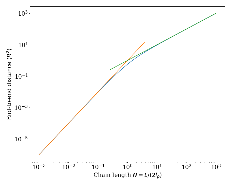
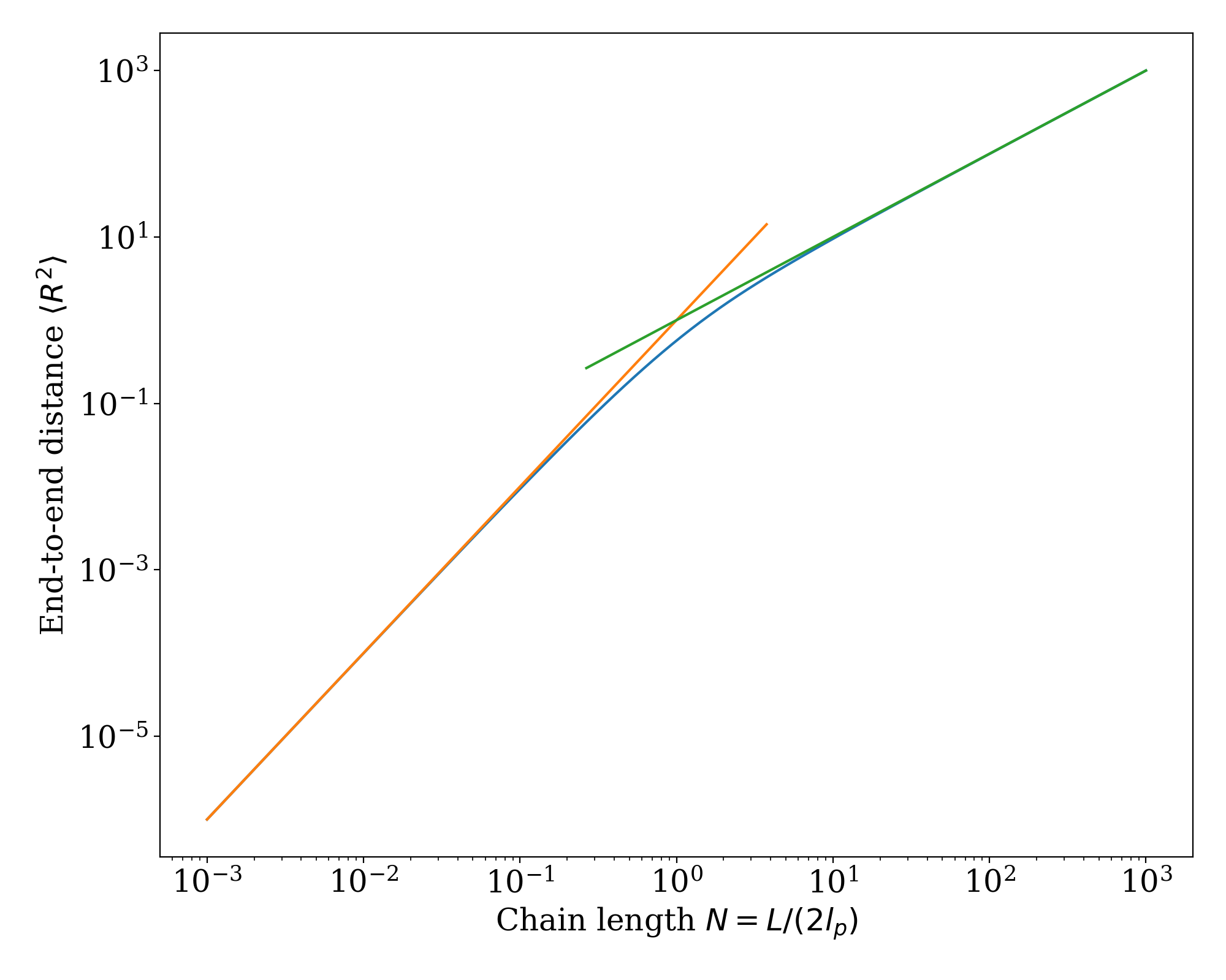
This example gives the mean-square end-to-end distance \(\langle R^{2} \rangle / (2 l_{p})^{2}\) (i.e. length non-dimensionalized by \(2 l_{p}\)) versus chain length \(N = L/(2 l_{p})\) for 3 dimensions. The short-length asymptotic behavior \(\langle R^{2} \rangle / (2 l_{p})^{2} \rightarrow N^{2}\) and long-length asymptotic behavior \(\langle R^{2} \rangle / (2 l_{p})^{2} \rightarrow 2 N/(d-1)\) are included to show the limiting behaviors.

(Source code, png, hires.png, pdf)

Example usage of ‘rg2_ave’

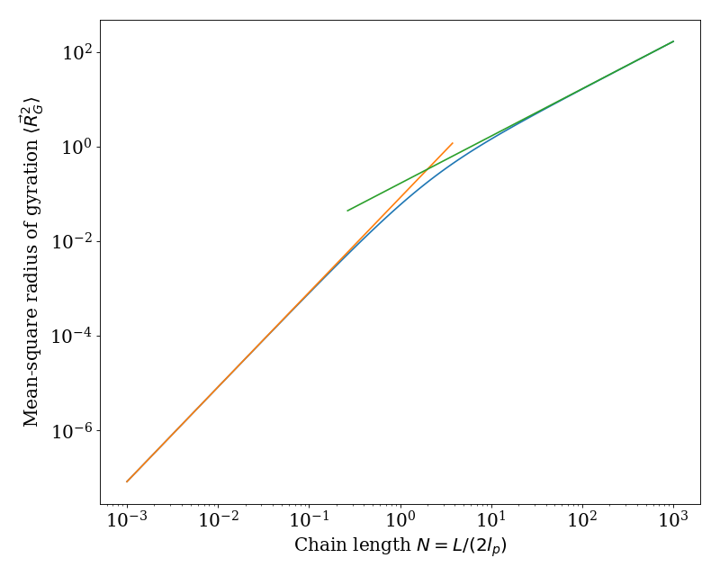
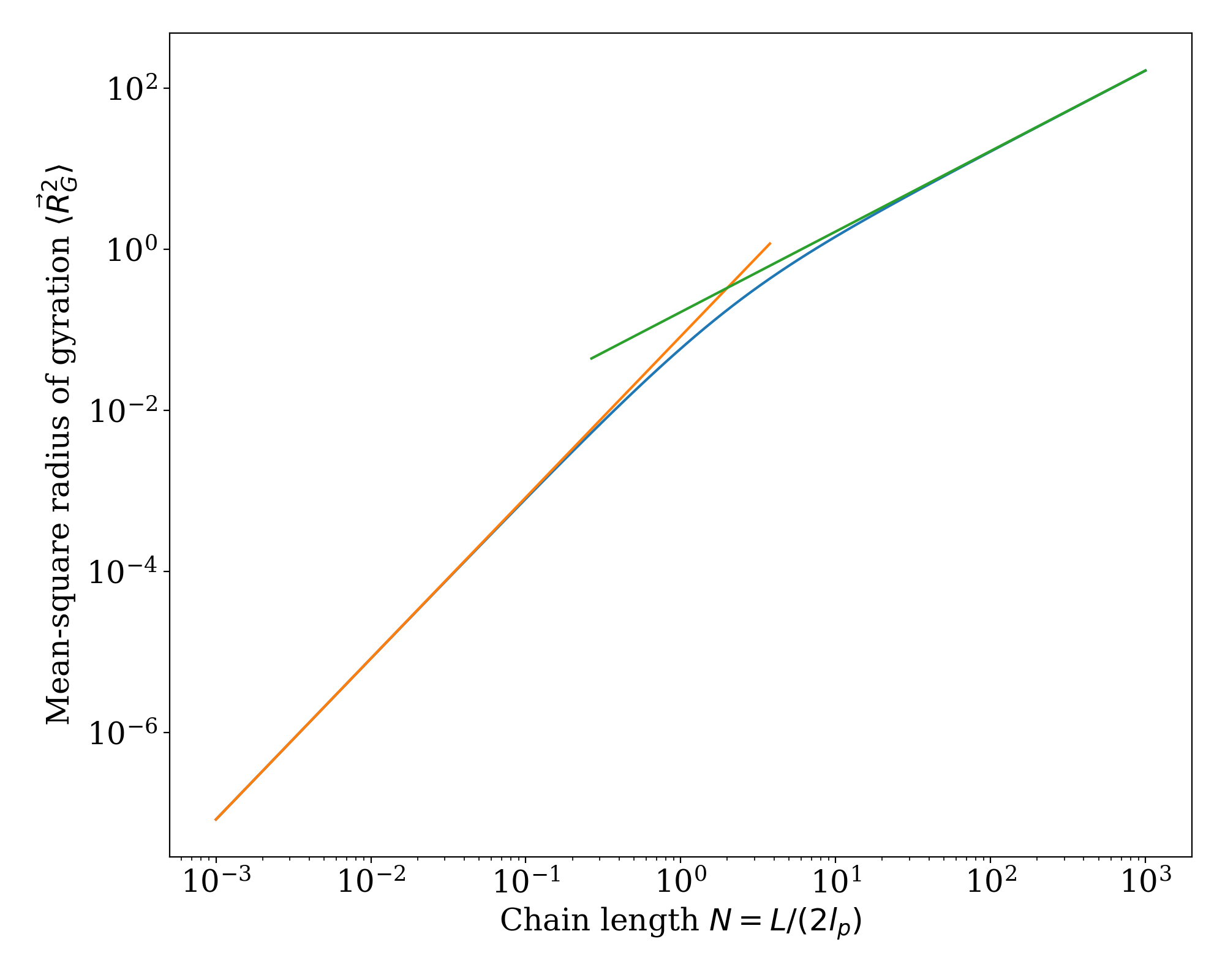
This example gives the mean-square radius of gyration \(\langle \vec{R}_{G}^{2} \rangle / (2 l_{p})^{2}\) (i.e. length non-dimensionalized by \(2 l_{p}\)) versus chain length \(N = L/(2 l_{p})\) for 3 dimensions. The short-length asymptotic behavior \(\langle \vec{R}_{G}^{2} \rangle / (2 l_{p})^{2} \rightarrow N^{2}/12\) and long-length asymptotic behavior \(\langle \vec{R}_{G}^{2} \rangle / (2 l_{p})^{2} \rightarrow N/[3 (d-1)]\) are included to show the limiting behaviors.

(Source code, png, hires.png, pdf)

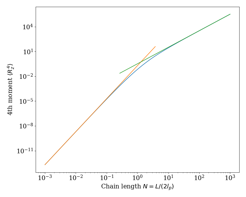
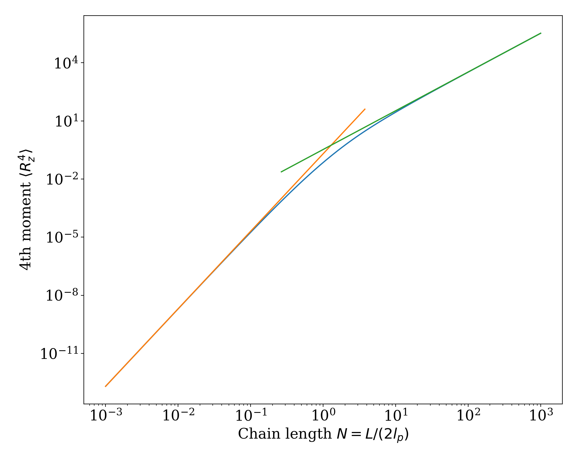
Example usage of ‘rz4_ave’

This example gives the 4th moment of the end-to-end distribution \(\langle R_{z}^{4} \rangle / (2 l_{p})^{4}\) (i.e. length non-dimensionalized by \(2 l_{p}\)) versus chain length \(N = L/(2 l_{p})\) for 3 dimensions. The short-length asymptotic behavior \(\langle R_{z}^{4} \rangle / (2 l_{p})^{2} \rightarrow N^{4} 3 / [d (d + 2)]\) and long-length asymptotic behavior \(\langle R_{z}^{4} \rangle / (2 l_{p})^{2} \rightarrow 12 N^2/[d^2 (d-1)^2]\) are included to show the limiting behaviors.

(Source code, png, hires.png, pdf)