Chromosomal DNA

We present a model ([Beltran2019]) combining thermal fluctuations in the DNA linkers with the geometric effects of experimentally-relevant linker length heterogeneity. We show that almost any linker length heterogeneity is sufficient to produce the disordered chromatin structures thatare now believed to dominate nuclear architecture. The intuition behind our structural claims extends to any polymer composed of aperiodic kinks, such as the dihedral “kinks” found at junctions of block copolymers.

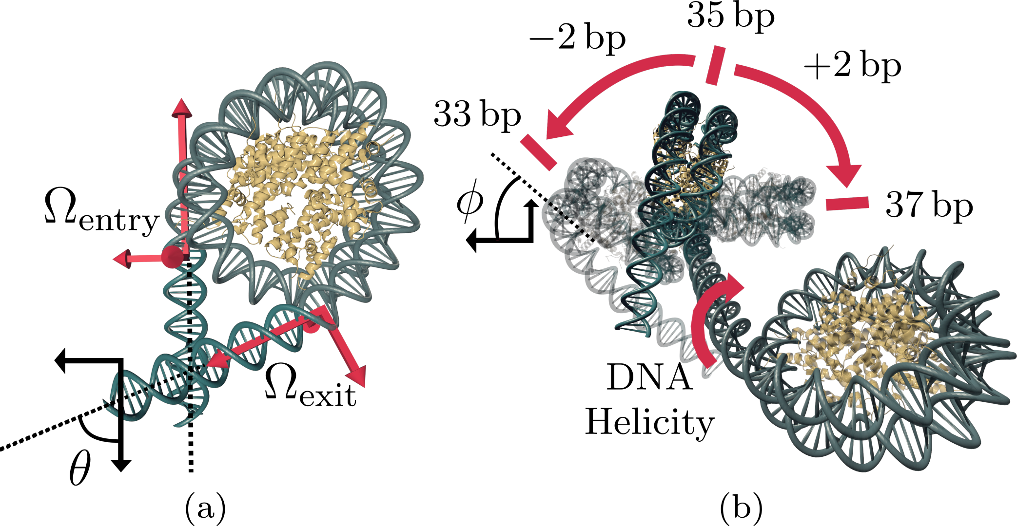
The structure of a nucleosome with straight linkers extrapolated from the entry (\(\Omega_\text{entry}\)) and exit (\(\Omega_\text{exit}\)) orientations of the bound DNA.

We model each DNA linker as a twistable wormlike chain (TWLC), and the nucleosomes as the points where these linker strands connect. We label the orientation of the DNA entering the i th nucleosome by the matrix \(\Omega^{(i)}_\text{entry}\). The exit orientation \(\Omega^{(i)}_\text{exit}\) must then satisfy \(\Omega^{(i)}_\text{exit} = \Omega^{(i)}_\text{entry} \cdot \Omega_\text{kink}\), where \(\Omega_\text{kink}\) is the fixed “kink” rotation.

We represent a TWLC of length \(L\) as a space curve \(\vec{R}(s)\), where \(0 < s < L\). The chain’s orientation at each point along this curve, \(\Omega(s)\), is represented by an orthonormal triad \(\vec{t}_{i}\), where \(\vec{t}_{3} = \partial_s \vec{R}(s)\). We track the bend and twist of our polymer via the angular “velocity” vector \(\vec{\omega}(s)\), which operates as \(\partial_s \vec{t}_{i}(s) = \vec{\omega}(s) \times \vec{t}_{i}(s)\). The Green’s function

\[G_{\text{TWLC}} (\vec{R}, \Omega | \Omega_0;L_1 ) =\! \int_{\Omega(0)=\Omega_0}^{\Omega(s)=\Omega} \hspace{-0.3in} \mathcal{D} [\Omega(s)] e^{-\beta \mathcal{E}}\delta(\vec{R} - \!\int_{0}^{L_1} \!\!\vec{t_3} ds),\]

of the first linker represents the probability that a polymer of length \(L_1\) that begins at the origin with initial orientation \(\Omega_0\) ends at position \(\vec{R}\) with end orientation \(\Omega\). For a TWLC with no kinks, the energy is quadratic in bending and twist deformations

\[\beta \mathcal{E} = \frac{l_p}{2}\int_{0}^{L_1} \!\ \! ds \, (\omega_1^2 + \omega_2 ^2) + \frac{l_t}{2}\int_{0}^{L_1} \! \! ds \, {\left(\omega_3 - \tau\right)}^2\]

The natural twist of DNA gives \(\tau = 2 \pi (\text{10.5} \, \text{bp})^{-1}\), and we set the persistence length \(l_p = 50 \, \text{nm}\) and twist persistence length \(l_t = 10 \, \text{nm}\) to match measurements of DNA elasticity.

Reference [Spakowitz2006] solves \(G_{\text{TWLC}}\) analytically in Fourier space (\(\vec{R} \rightarrow \vec{k}\)) by computing the coefficients of the Wigner D-function expansion

\[\hat{G} (\vec{k}, \Omega | \Omega_0;L_1 ) = \sum_{\substack{ l;\hspace{0.1em}l_0 m_0 j_0}} \!\! g_{l_0 m_{0} j_{0}}^{l m_0 j_0} \mathcal{D}_{l}^{m_0j_0}(\Omega) \mathcal{D}_{l_0}^{m_0 j_0 *}(\Omega_0).\]

To account for \(\Omega_\text{kink}\), we rotate the final orientation of the linker DNA, \(\Omega = \Omega_\text{entry}\), to \(\Omega_\text{exit}\) using the formula

\[\mathcal{D}_l^{m_0j_0}(\Omega \cdot \Omega_\text{kink}) = \sum_j \sqrt{\frac{8\pi}{2l+1}} \mathcal{D}_l^{m_0j}(\Omega_\text{kink}) \mathcal{D}_l^{jj_0}(\Omega).\]

The resulting Green’s function combines the effects of a DNA linker and a nucleosome, but is still a Wigner D-function expansion with modified coefficients \(B_{l_{0} m_{0} j_{0}}^{l m_0 j}\).

Functions contained with the ‘chromo’ module

Kinked WLC with twist and fixed ends

This module calculates statistics for a series of worm-like chains with twist (DNA linkers) connected by kinks imposed by nucleosomes. Calculations include R^2, Kuhn length, propogator matrices, full Green’s function for the end-to-end distance of the polymer, and looping statistics.

Code written by Bruno Beltran, Deepti Kannan, and Andy Spakowitz

wlcstat.chromo.H(i, r, c, T, b)

Parametric description of a simple left-handed helix aligned with \(\hat{z}\).

The helix is parametrized on [0,1]. Has height c, radius r, and undergoes T twists in that range. Centerline is the positive z-axis and starting point is (r,0,0).

Parameters

${helix_doc} –

Returns

X – Position coordinate for each i.

Return type

(3,N) np.ndarray

wlcstat.chromo.H_oriented(*args, **kwargs)

Position a helix at entry_pos and entry_rot, as returned by e.g. minimum_energy_no_sterics.

Parameters

• ${helix_doc} –

• ${orientation_doc} –

Returns

X – Position coordinate for each i.

Return type

(3,N) np.ndarray

wlcstat.chromo.H_rot(i, r, c, T, b)

OmegaH(s). Given OmegaH(0) = [Hn, Hb, Hu].

A rotation element, so det(H_rot) == 1.

wlcstat.chromo.H_rot_oriented(*args, **kwargs)

OmegaH(s) given OmegaH(0) arbitrary.

A rotation element, so det(H_rot) == 1. For some reason, tends to produce matrices that are numerically off of H_rot by a factor of like 1-2% in each element for equivalent parameters? Off by one somewhere? That’s the order of magnitude of a bp.

wlcstat.chromo.Hb(*args, **kwargs)

Bi-normal vector to H(). Unit vector in the direction of \(\frac{dH}{di}\times\frac{d^2 H}{di^2}\).

Parameters

• ${helix_doc} –

• ${normed_doc} –

Returns

B – Bi-normal vector for each i.

Return type

(3,N) np.ndarray

wlcstat.chromo.Hk(r, c, T, b)

Curvature of our standard helix.

Parameters

${helix_params_doc} –

Returns

k – Curvature of the helix.

Return type

float64

Notes

The curvature of a helix is a constant, in our parameterization it works out to \(\frac{r}{\gamma}\left(\frac{2\pi T}{b}\right)^2\), where \(\gamma = (1/b)\sqrt{4\pi^2r^2T^2 + c^2}\).

wlcstat.chromo.Hn(i, r, c, T, b, normed=True)

Normal vector to H(). The unit vector in the direction of \(\frac{d^2 H}{di^2}\).

Parameters

• ${helix_doc} –

• ${normed_doc} –

Returns

N – Normal vector for each i.

Return type

(3,N) np.ndarray

wlcstat.chromo.Hn_oriented(*args, **kwargs)

Normal to H_oriented() at entry_rot.

Parameters

• ${helix_params_doc} –

• ${entry_rot_doc} –

Returns

n – normal vector for each i.

Return type

(3,N) np.ndarray

wlcstat.chromo.Htau(r, c, T, b)

Torsion of our standard helix.

Parameters

${helix_params_doc} –

Returns

tau – Torsion of the helix.

Return type

float64

Notes

The torsion of a helix is a constant, in our parameterization it works out to \(\frac{-2\pi c T}{b} \left[4\pi^2r^2T^2 + c^2\right]^{-1/2}\).

wlcstat.chromo.Hu(i, r, c, T, b, normed=True)

Tangent vector to H(), \(\frac{dH}{di}\).

Parameters

• ${helix_doc} –

• ${normed_doc} –

Returns

U – Tangent vector for each i.

Return type

(3,N) np.ndarray

wlcstat.chromo.Hu_oriented(*args, **kwargs)

Tangent to H_oriented() at entry_rot.

Parameters

• ${helix_params_doc} –

• ${entry_rot_doc} –

Returns

U – Tangent vector for each i.

Return type

(3,N) np.ndarray

wlcstat.chromo.OmegaC(Lw, helix_params={'T': 1.8375, 'b': 147, 'c': 4.531142964071856, 'r': 4.1899999999999995})

inv(H_rot(0)) @ H_rot(Lw)

The non-twist-corrected rotation matrix that takes the n, b, and u vectors of the helix from the start of the helix to the exit.

Parameters

• Lw (float) – Length of DNA bound to the nucleosome (#bound bp - 1)

• helix_params ((optional) Dict[str, float]) –

Returns

Omega_next – Rotation matrix taking the input to output orientations of the normal, binormal, tangent triad of the helix.

Return type

(3, 3) np.ndarray[float64]

wlcstat.chromo.OmegaE2E(Lw=146, *, tau_n=0.6178156644227715, helix_params={'T': 1.8375, 'b': 147, 'c': 4.531142964071856, 'r': 4.1899999999999995})

Nucleosome core entry to exit rotation matrix \(\Omega_C \cdot R_z(L_w \left[ \tau_n - \tau_H \right])\) Should be multiplied against entry orientation from the right to get the exit orientation.

Example

To get the exit orientation from the nucleosome assuming the bound DNA adopts a configuration with zero intrinsic twist is just >>> import nuc_chain.geometry as ncg >>> Omega0 = np.identity(3) >>> Omega0Exit = Omega0 @ ncg.OmegaE2E(tau_n=0)

Parameters

• tau_n (float) – the twist density of nucleosome-bound dna in radians/bp

• Lw (float) – Length of DNA bound to the nucleosome (#bound bp - 1)

• helix_params (Dict[str, float]) – parameters to H() family of function

Returns

• OmegaE2E ((3,3) np.ndarray[float64])

• Entry to exit rotation matrix

wlcstat.chromo.OmegaNextAssoc(Ll, *, w_in=73, w_out=73, tau_n=0.6178156644227715, tau_d=0.5983986006837702, helix_params={'T': 1.8375, 'b': 147, 'c': 4.531142964071856, 'r': 4.1899999999999995})

Nucleosome entry to exit (including unwrapped DNA on both sides).

wlcstat.chromo.OmegaNextEntry(Ll, *, w_in=73, w_out=73, tau_n=0.6178156644227715, tau_d=0.5983986006837702, helix_params={'T': 1.8375, 'b': 147, 'c': 4.531142964071856, 'r': 4.1899999999999995})

Nucleosome entry to entry.

wlcstat.chromo.OmegaNextExit(Ll, *, w_in=73, w_out=73, tau_n=0.6178156644227715, tau_d=0.5983986006837702, helix_params={'T': 1.8375, 'b': 147, 'c': 4.531142964071856, 'r': 4.1899999999999995})

Nucleosome exit to exit.

wlcstat.chromo.Rx(theta)

Rotation matrix about the x axis with angle theta.

Notes

..math:

\frac{1}{\sqrt{3}}
\begin{bmatrix}
    1 &             0 &              0\\
    0 & np.cos(theta) & -np.sin(theta)\\
    0 & np.sin(theta) &  np.cos(theta)
\end{bmatrix}

wlcstat.chromo.Ry(theta)

Rotation matrix about the z axis with angle theta.

Notes

..math:

\frac{1}{\sqrt{3}}
\begin{bmatrix}
    np.cos(theta) & 0 & -np.sin(theta) \\
                0 & 1 &              0 \\
    np.sin(theta) & 0 &  np.cos(theta)
\end{bmatrix}

wlcstat.chromo.Rz(theta)

Rotation matrix about the z axis with angle theta.

Notes

..math:

\frac{1}{\sqrt{3}}
\begin{bmatrix}
    np.cos(theta) & -np.sin(theta) & 0 \\
    np.sin(theta) &  np.cos(theta) & 0 \\
                0 &             0  & 1
\end{bmatrix}

wlcstat.chromo.build_B_matrices_for_R2(link, alpha, beta, gamma, lt=301.2048192771084, lp=150.6024096385542, tau_d=0.5983986006837702, lmax=2)

Helper function to construct propogator B matrices for a single linker length link with kink rotation given by alpha, beta, gamma. Returns the following three matrices:

\[B^{(n)} = \lim_{k \to 0}\frac{d^n B}{dk^n}\]

for n = 0, 1, and 2. where B is defined as

\[B^{l_f j_f}_{l_0 j_0} = \sqrt{\frac{8\pi^2}{2l_f+1}} {\mathcal{D}}^{j_f j_0}_{l_f}(-\gamma, -\beta, -\alpha) g^{j_0}_{l_f l_0} B^{(n)}[I_f, I_0] = M[I_f, I_0] * g^{(n)}[I_f, I_0]\]

The g matrix is used for the linker propogator, and the M matrix represents the rotation due to the kink. All matrices are super-indexed by B[If, I0] where \(I(l, j) = l^2 + l + j\). \(I\) can take on \(l^2+2l+1\) possible values.

Notes

Andy adds 1 to the above formula for \(I\) since his script is in Matlab, which is one-indexed.

Parameters

• link (float) – linker length in bp

• lt (float) – twist persistence length in bp

• lp (float) – DNA persistence length in bp

• tau_d (float) – twist density of naked DNA in rad/bp

• lmax (int) – maximum eigenvalue l for which to compute wigner D’ (default lmax = 2)

Returns

[B0, B1, B2] – list of 3 matrices, each of dimension \(l_{max}^2 + 2l_{max} + 1\)

Return type

(3,) list

wlcstat.chromo.gen_chromo_conf(links, lt=301.2048192771084, lp=150.6024096385542, kd_unwrap=None, w_ins=73, w_outs=73, tau_d=0.5983986006837702, tau_n=0.6178156644227715, lpb=0.332, r_dna=1.0, helix_params={'T': 1.8375, 'b': 147, 'c': 4.531142964071856, 'r': 4.1899999999999995}, unwraps=None, random_phi=False)

Generate DNA and nucleosome conformation based on chain growth algorithm

Parameters

• links ((L,) array-like) – linker length in bp

• w_ins (float or (L+1,) array_like) – amount of DNA wrapped on entry side of central dyad base in bp

• w_outs (float or (L+1,) array_like) – amount of DNA wrapped on exit side of central dyad base in bp

• tau_n (float) – twist density of nucleosome-bound DNA in rad/bp

• tau_d (float) – twist density of naked DNA in rad/bp

• lt (float) – twist persistence length in bp

• lp (float) – DNA persistence length in bp

wlcstat.chromo.gen_chromo_pymol_file(r, rdna1, rdna2, rn, un, filename='r_poly.pdb', ring=False)

Parameters

• r –

• rdna1 –

• rdna2 –

• rn –

• un –

• filename –

• ring –

wlcstat.chromo.kvals = array([0.00000000e+00, 3.32000000e-06, 3.32612191e-06, ..., 3.31966798e+02, 3.31983399e+02, 3.32000000e+02])

Good values to use for integrating our Green’s functions. If the lp of the bare chain under consideration changes, these should change.

wlcstat.chromo.minimum_energy_no_sterics_linker_only(links, *, w_ins=73, w_outs=73, tau_n=0.6178156644227715, tau_d=0.5983986006837702, lpb=0.332, helix_params={'T': 1.8375, 'b': 147, 'c': 4.531142964071856, 'r': 4.1899999999999995}, unwraps=None, random_phi=None)

Calculate the theoretical conformation of a chain of nucleosomes connected by straight linkers (ground state) with no steric exclusion.

Parameters

• links ((L,) array_like) – lengths of each linker segment

• tau_n (float) – twist density of nucleosome-bound DNA in rad/bp

• tau_d (float) – twist density of linker DNA in rad/bp

• w_ins (float or (L+1,) array_like) – amount of DNA wrapped on entry side of central dyad base

• w_outs (float or (L+1,) array_like) – amount of DNA wrapped on exit side of central dyad base

Returns

• entry_rots ((L+1,3,3) np.ndarray) – the orientation of the material normals (as columns) of the DNA at the entry site

• entry_pos ((L+1,3) np.ndarray) – the position of the entry site of each nucleosome (where the first bp is bound)

wlcstat.chromo.normalize_HX(X)

Normalize a list of 3-vectors of shape (N,3).

Parameters

X ((N, 3) array_like) – N input vectors to be normalized.

Returns

U – N outputs, such that np.linalg.norm(U[i,:]) == 1 for i in range N.

Return type

(N, 3) np.ndarray

wlcstat.chromo.r2_kinked_twlc(links, lt=301.2048192771084, lp=150.6024096385542, kd_unwrap=None, w_ins=73, w_outs=73, tau_d=0.5983986006837702, tau_n=0.6178156644227715, lmax=2, helix_params={'T': 1.8375, 'b': 147, 'c': 4.531142964071856, 'r': 4.1899999999999995}, unwraps=None, random_phi=False)

Calculate the mean squared end-to-end distance, or \(\langle{R^2}\rangle\) of a kinked WLC with a given set of

linkers and unwrapping amounts.

Parameters

• links ((L,) array-like) – linker length in bp

• w_ins (float or (L+1,) array_like) – amount of DNA wrapped on entry side of central dyad base in bp

• w_outs (float or (L+1,) array_like) – amount of DNA wrapped on exit side of central dyad base in bp

• tau_n (float) – twist density of nucleosome-bound DNA in rad/bp

• tau_d (float) – twist density of naked DNA in rad/bp

• lt (float) – twist persistence length in bp

• lp (float) – DNA persistence length in bp

• lmax (int) – maximum eigenvalue l for which to compute wigner D’ (default lmax = 2)

Returns

• r2 ((L,) array-like) – mean square end-to-end distance of kinked chain as a function of chain length in nm^2

• ldna ((L,) array-like) – mean square end-to-end distance of kinked chain as a function of chain length in nm

• kuhn (float) – Kuhn length as defined by \(\langle{R^2}\rangle / R_{max}\) in long chain limit

wlcstat.chromo.resolve_wrapping_params(unwraps, w_ins=None, w_outs=None, N=None, unwrap_is='bp')

Allow the user to specify either one value (and tile appropriately) or an array of values for the number of base pairs bound to the nucleosome. Also allow either the number of base pairs bound on each side of the dyad to be specified or the number of base pairs unwrapped relative to the crystal structure (in which case the unwrapping is split evenly on either side of the dyad for simplicity.

Parameters

• unwraps (float or (N,) array_like) – total amount of unwrapped DNA on both sides

• (optional) (N) – wrapped DNA on entry side of dyad axis

• (optional) – wrapped DNA on exit side of dyad axis

• (optional) – output size, if other params are not array_like

• unwrap_is (string) – ‘bp’ or ‘sites’, to specify whether we’re counting the number of bp bound or the number of nucleosome-to-dna contacts (respectively)

Returns

• w_in ((N,) np.ndarray) – N output wrapping lengths on entry side of dyad axis

• w_out ((N,) np.ndarray) – N output wrapping lengths on exit side of dyad axis

• All functions take w_in, w_out directly now.

wlcstat.chromo.zyz_from_matrix(R)

Convert from a rotation matrix to (extrinsic zyz) Euler angles.

Parameters

R ((3, 3) array_like) – Rotation matrix to convert

Returns

• alpha (float) – The final rotation about z’’

• beta (float) – The second rotation about y’

• gamma (float) – the initial rotation about z

Notes

See pg. 13 of Bruno’s (NCG) nucleosome geometry notes for a detailed derivation of this formula. Easy to test correctness by simply reversing the process R == Rz(alpha)@Ry(beta)@Rz(gamma).

Example usage of ‘r2_kinked_twlc’

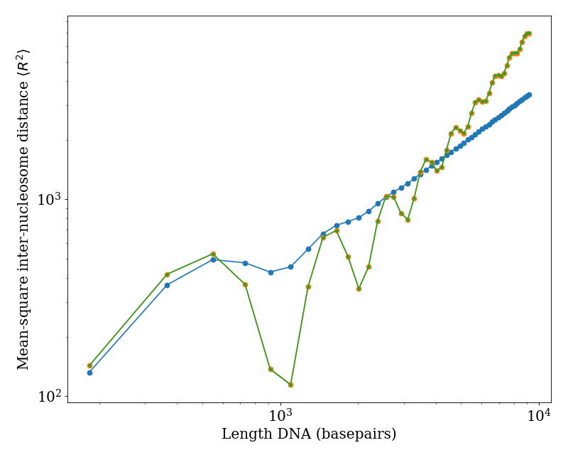
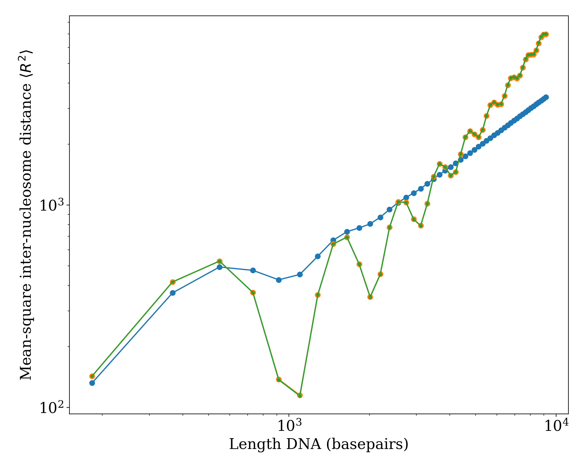
We plot the mean-square inter-nucleosome distance \(\langle R^{2} \rangle\) versus total DNA length (i.e. including both linker DNA and nucleosomal DNA) for a fixed linker length of 36 basepairs. The blue points show predictions using standard physical properties of DNA [\(l_{p} = 50 \, \text{nm}\), \(l_{t} = 100 \, \text{nm}\), \(\tau = 2 \pi / (10.5 \, \text{basepairs})\)]. The orange and green curves show zero temperature predictions (i.e. no conformation fluctuations) using the ‘r2_kinked_twlc’ code in the limit of \(l_{p}, l_{t} \gg 1\) (orange) and using a straight-linker algorithm (green), demonstrating quantitative agreement between these approaches.

(Source code, png, hires.png, pdf)

Example usage of ‘gen_chromo_conf’ and ‘gen_chromo_pymol_file’

We demonstrate the usage of ‘gen_chromo_conf’ to generate the conformation of a chromosome array with 100 nucleosomes and random linker lengths between 35 and 50 basepairs. The output conformation is used to generate a PyMOL file using ‘gen_chromo_pymol_file’. The resulting file ‘r_chromo.pdb’ is loaded in PyMOL to generate an image of the chromosomal DNA.

links = np.random.randint(35, 50, 100)
r, rdna1, rdna2, rn, un = gen_chromo_conf(links)
gen_chromo_pymol_file(r, rdna1, rdna2, rn, un, filename='r_chromo.pdb', ring=False)

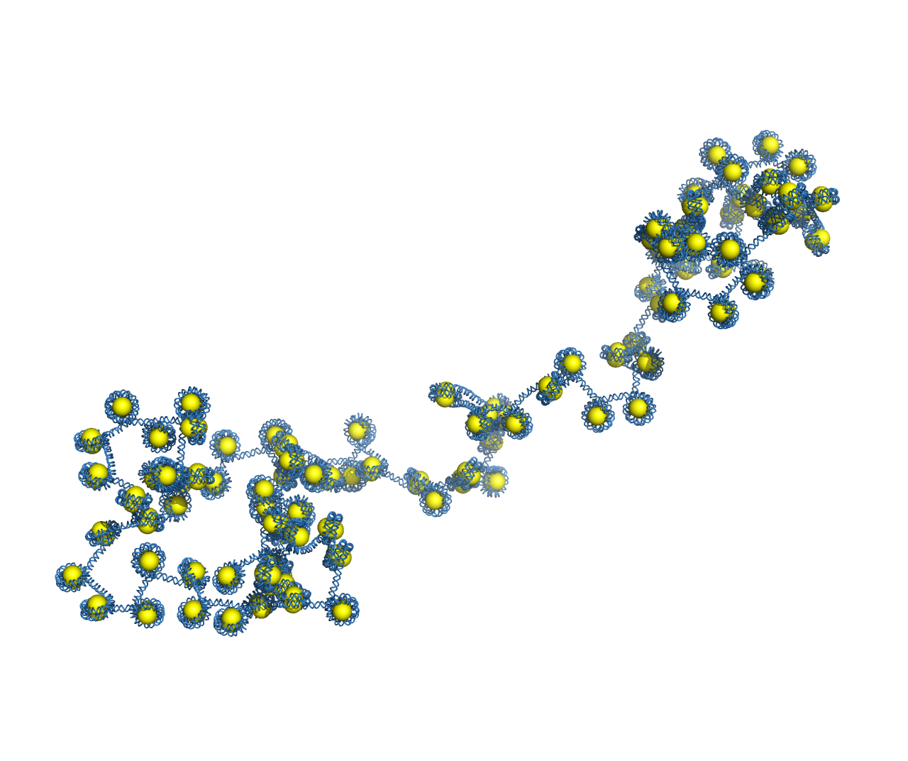
Image of a 100-nucleosome array generated in PyMOL using output from ‘gen_chromo_conf’ and ‘gen_chromo_pymol_file’.