Wormlike Chains with Twist, Helices, and Ribbons

Polymer chain representations

The conformation of a polymer chain can be defined by either an all-atom representation or an effective-chain representation. For a polymer of any appreciable molecular weight, an all-atom representation is impractical for analytical theory and is computationally limited to short time scales. Here, we will focus on effective-chain representations in order to develop theoretical descriptions that can address length and time scales relevant to biological processes.

Definition of effective-chain representation

Define the space curve \(\vec{r}(s)\) with pathlength variable \(s\) that runs from \(0\) at one end of the chain to \(L\) at the other end. Define the unit tangent vector \(\vec{u}(s)\) to be

\[\vec{u}(s) = \frac{1}{\gamma(s)} \frac{\partial \vec{r}(s)}{\partial s},\]

where

\[\gamma(s) = \left| \frac{\partial \vec{r}(s)}{\partial s} \right|.\]

The local curvature of the chain is defined by

\[\frac{\partial \vec{u}(s)}{\partial s} = \frac{1}{\gamma} \left( \mathbf{I} - \vec{u} \vec{u} \right) \cdot \frac{\partial^{2} \vec{r}}{\partial s^{2}} =\kappa (s) \vec{n}(s),\]

where \(\vec{n}(s)\) is the curve normal at \(s\) (note, \(\vec{n} \cdot \vec{u} = 0\)), and \(\kappa(s)\) is the local curvature of the curve (note, \(\kappa(s) \ge 0\)). The local curvature \(\kappa\) is related to the radius \(R\) of a circle that is drawn tangent to the curve, such that \(R = \kappa^{-1}\). Define the unit binormal to the curve \(\vec{b}=\vec{u} \times \vec{n}\) to define a unit triad to the space curve, i.e.

\[\begin{split}& & \vec{u} \cdot \vec{u} = 1, \hspace{0.1in} \vec{n} \cdot \vec{n} = 1, \hspace{0.1in} \vec{b} \cdot \vec{b} = 1, \hspace{0.1in} \nonumber \\ & & \vec{u} \cdot \vec{n} = 0, \hspace{0.1in} \vec{u} \cdot \vec{b} = 0, \hspace{0.1in} \vec{n} \cdot \vec{b} = 0 \hspace{0.1in}\end{split}\]

Our current representation does not include an internal degree of freedom associated with the twisting of the chain. %which is important for a variety of applications Define a unit triad to the curve \(\vec{t}_{i}\) (\(i=1,2,3\)), where \(\vec{t}_{i} \cdot \vec{t}_{j} = \delta_{ij}\) and \(\vec{t}_{i} = \epsilon_{ijk} \vec{t}_{j} \times \vec{t}_{k}\). The tangent vector is aligned with \(\vec{t}_{3}\), thus \(\vec{u} = \vec{t}_{3}\). Define the rotation vector \(\vec{\omega}\) such that \(\frac{\partial \vec{t}_{i}}{\partial s} = \vec{\omega} \times \vec{t}_{i}\), or

\[\frac{\partial \vec{t}_{1}}{\partial s} = \omega_{3} \vec{t}_{2} - \omega_{2} \vec{t}_{3}, \hspace{0.2in} \frac{\partial \vec{t}_{2}}{\partial s} = \omega_{1} \vec{t}_{3} - \omega_{3} \vec{t}_{1}, \hspace{0.2in} \frac{\partial \vec{t}_{3}}{\partial s} = \omega_{2} \vec{t}_{1} - \omega_{1} \vec{t}_{2}\]

This representation is related to the previous representation as \(\kappa = \sqrt{\omega_{1}^{2}+\omega_{2}^{2}}\) and \(\vec{n} = \frac{\omega_{2}}{\sqrt{\omega_{1}^{2}+\omega_{2}^{2}}} \vec{t}_{1} - \frac{\omega_{1}}{\sqrt{\omega_{1}^{2}+\omega_{2}^{2}}} \vec{t}_{2}\)

Definition of effective-chain representation including internal twist degree of freedom

Geometry and topology of space curves

Geometric quantities

The geometry of a single curve is described by the space curve \(\vec{r}(s)\). The local deformation of the chain from a straight conformation described by the curvatures \(\omega_{i}\), where \(\omega_{1}\) and \(\omega_{2}\) are bend curvatures (related to \(\kappa\)) and \(\omega_{3}\) is the twist curvature. Another geometric quantity called the torsion \(\tau\) describes the ``out-of-planeness” of the curve, where

\[\frac{\partial \vec{b}}{\partial s} = \vec{u} \times \frac{\partial \vec{n}}{\partial s} + \frac{\partial \vec{u}}{\partial s} \times \vec{n} = \vec{u} \times \frac{\partial \vec{n}}{\partial s} = - \tau \vec{n}.\]

For example, consider a regular helix with space curve

\[\vec{r}(s) = a \cos \! \left( \frac{2 \pi s}{l_{t}} \right) \hat{x} + a \sin \! \left( \frac{2 \pi s}{l_{t}} \right) \hat{y} + h \frac{s}{l_{t}} \hat{z}\]

where \(a\) is the helix radius, \(l_{t}\) is the length per helix turn, and \(h\) is the height per helix turn. To fix \(\gamma=1\) for all \(s\), we fix \(l_{t}=\sqrt{(2 \pi)^{2} a^{2} + h^{2}}\). This condition makes \(s\) an arclength parameter that constrains the chain length of the curve.

This chain conformation results in

\[\begin{split}& & \vec{u} = - \frac{2 \pi a}{l_{t}} \sin \! \left( \frac{2 \pi s}{l_{t}} \right) \hat{x} + \frac{2 \pi a}{l_{t}} \cos \! \left( \frac{2 \pi s}{l_{t}} \right) \hat{y} + \frac{h}{l_{t}} \hat{z} \nonumber \\ & & \vec{n} = - \cos \! \left( \frac{2 \pi s}{l_{t}} \right) \hat{x} - \sin \! \left( \frac{2 \pi s}{l_{t}} \right) \hat{y} \nonumber \\ & & \vec{b} = \frac{h}{l_{t}} \sin \! \left( \frac{2 \pi s}{l_{t}} \right) \hat{x} - \frac{h}{l_{t}} \cos \! \left( \frac{2 \pi s}{l_{t}} \right) \hat{y} + \frac{2 \pi a}{l_{t}} \hat{z}.\end{split}\]

This results in a constant curvature and torsion

\[\kappa = \frac{(2 \pi)^{2} a}{(2 \pi)^{2} a^{2} + h^{2}} \hspace{0.2in} \mathrm{and} \hspace{0.2in} \tau = \frac{2 \pi h}{(2 \pi)^{2} a^{2} + h^{2}}\]

As \(h \rightarrow 0\), the curvature is \(\kappa = 1/a\), where \(a\) is the radius of the flattened circle, and \(\tau=0\) due to the planar conformation. As \(a \rightarrow 0\), the curvature \(\kappa\) is zero, and the torsion \(\tau = 2 \pi/h\). The torsion is only mathematically defined in this limit due to the underlying definition of the helix. Such geometric quantities are sensitive to the local chain conformation and do not define global properties of the chain. Chain topology is defined through quantities that define the global state of the chain and are insensitive to local geometric changes

Topological quantities

Topological quantities are typically defined for closed curves, i.e. curves whose ends are joined together into a closed ring. Consider a smooth, closed curve whose ends are continuous, thus \(\frac{\partial^{n} \vec{r}(s=0)}{\partial s^{n}}= \frac{\partial^{n} \vec{r}(s=L)}{\partial s^{n}}\) for all \(n\). First consider a 2-D curve and ask how many times this curve wraps around the origin, defined as the Winding Number \(Wi\). Defining the space curve in polar coordinates \(\vec{r}(s) = r(s) \cos \theta(s) \hat{x}+ r(s) \sin \theta(s) \hat{y}\), we have

\[Wi = \frac{1}{2 \pi} \left[ \theta(s=L)-\theta(s=0) \right]= \frac{1}{2 \pi} \int_{0}^{L} \! \! ds \, \frac{\partial \theta(s)}{\partial s}.\]

Schematic of the Winding Number \(Wi\) (in 2 dimensions) of various curves (see http://en.wikipedia.org/wiki/Winding_,number)

The Winding Number is related to \(\vec{r}(s)\) through

\[\begin{split}& & \frac{\partial \vec{r}}{\partial s} = \left( \frac{\partial r}{\partial s} \cos \theta - r \sin \theta \frac{\partial \theta}{\partial s} \right) \hat{x}+ \left( \frac{\partial r}{\partial s} \sin \theta + r \cos \theta \frac{\partial \theta}{\partial s} \right) \hat{y} \nonumber \\ & & \frac{\partial \vec{r}}{\partial s} \times \hat{z} = %\times \frac{\partial \vec{r}}{\partial s} = \left( \frac{\partial r}{\partial s} \sin \theta + r \cos \theta \frac{\partial \theta}{\partial s} \right) \hat{x} - \left( \frac{\partial r}{\partial s} \cos \theta - r \sin \theta \frac{\partial \theta}{\partial s} \right) \hat{y} \nonumber \\ & & \frac{\partial \theta}{\partial s}= \frac{\vec{r}}{\left| \vec{r} \right|^{2}} \cdot \left( \frac{\partial \vec{r}}{\partial s} \times \hat{z} \right) \hspace{0.1in} \mathrm{thus} \hspace{0.1in} Wi = \frac{1}{2 \pi} \int_{0}^{L} \! \! ds \, \frac{\vec{r}}{\left| \vec{r} \right|^{2}} \cdot \left( \frac{\partial \vec{r}}{\partial s} \times \hat{z} \right).\end{split}\]

Now consider two closed curves in 3-D, defined by the space curves \(\vec{r}_{1}(s_{1})\) and \(\vec{r}_{2}(s_{2})\). Define the Linking Number \(Lk\) that gives the number of times the two curves wind around each other. This quantity is invariant to changes, provided you do not pass the curves through each other.

Schematic of the Linking Number \(Lk\) of various curve pairs (see http://en.wikipedia.org/wiki/Linking_,number)

Mathematically, the Linking Number is defined as

\[Lk = \frac{1}{4 \pi} \int_{0}^{L} \! \! ds_{1} \int_{0}^{L} \! \! ds_{2} \frac{\left( \vec{r}_{1}(s_{1})-\vec{r}_{2}(s_{2}) \right)} {\left| \vec{r}_{1}(s_{1})-\vec{r}_{2}(s_{2}) \right|^{3}} \cdot \left( \frac{\partial \vec{r}_{1}(s_{1})}{\partial s_{1}} \times \frac{\partial \vec{r}_{2}(s_{2})}{\partial s_{2}} \right),\]

which is essentially the 3-D extension of the winding number of curve one around curve 2, summed over curve 2. Although the Linking Number is a topological invariant for two curves that are entangled, a non-zero Linking Number is not a unique designation of entanglement, i.e. \(Lk=0\) does not necessarily mean the curves are not entangled.

Two examples where \(Lk=0\), but the curves are exhibit entanglement (see http://en.wikipedia.org/wiki/Linking_,number)

Knot theory provides further classifications for self-knotting and entanglement between multiple rings. Other topological quantities are used for knot classification.

Knot classification of 1, 2, and 3 rings

Now consider the self-linking of a curve by defining the first curve \(\vec{r}_{1}(s_{1})=\vec{r}(s_{1})\) and the second curve \(\vec{r}_{2}(s_{2})=\vec{r}(s_{2}) + \epsilon \vec{t}_{1}(s_{2})\), which winds around the first curve with the material normal \(\vec{t}_{1}\). The Linking Number between these curves is

\[\begin{split}Lk & = & \color{red}{ \frac{1}{4 \pi} \int_{0}^{L} \! \! ds_{1} \int_{0}^{L} \! \! ds_{2} \frac{\left( \vec{r}(s_{1})-\vec{r}(s_{2}) - \epsilon \vec{t}_{1}(s_{2}) \right)} {\left| \vec{r}(s_{1})-\vec{r}(s_{2}) - \epsilon \vec{t}_{1}(s_{2}) \right|^{3}} \cdot \left( \vec{t}_{3}(s_{1}) \times \vec{t}_{3}(s_{2}) \right)} \nonumber \\ & & + \color{blue}{ \frac{1}{4 \pi} \int_{0}^{L} \! \! ds_{1} \int_{0}^{L} \! \! ds_{2} \frac{\epsilon \left( \vec{r}(s_{1})-\vec{r}(s_{2}) - \epsilon \vec{t}_{1}(s_{2}) \right)} {\left| \vec{r}(s_{1})-\vec{r}(s_{2}) - \epsilon \vec{t}_{1}(s_{2}) \right|^{3}} \cdot \left( \vec{t}_{3}(s_{1}) \times \frac{\partial \vec{t}_{1}(s_{2})}{\partial s_{2}} \right)} \nonumber \\ & = & \color{red}{Wr} \color{black}{+} \color{blue}{Tw},\end{split}\]

where \(\color{red}{Wr}\) is a topological quantity called the Writhe, and \(\color{blue}{Tw}\) is a topological quantity called the Twist. In the limit \(\epsilon \rightarrow 0\), the Writhe \(Wr\) approaches

\[Wr = \frac{1}{4 \pi} \int_{0}^{L} \! \! ds_{1} \int_{0}^{L} \! \! ds_{2} \frac{\left( \vec{r}(s_{1})-\vec{r}(s_{2}) \right)} {\left| \vec{r}(s_{1})-\vec{r}(s_{2}) \right|^{3}} \cdot \left( \vec{t}_{3}(s_{1}) \times \vec{t}_{3}(s_{2}) \right).\]

As \(\epsilon \rightarrow 0\), the Twist \(Tw\) appears to approach zero. However, the integrand diverges as \(s_{2} \rightarrow s_{1}\), leading to a non-zero limiting value for the Twist \(Tw\). Note that \(\frac{\partial \vec{t}_{1}(s_{2})}{\partial s_{2}}= \omega_{3}(s_{2})\vec{t}_{2}(s_{2})- \omega_{2}(s_{2})\vec{t}_{3}(s_{2})\) and \(\vec{t}_{3} \times \vec{t}_{2} = - \vec{t}_{1}\).

The only part of the Twist \(Tw\) that will contribute as \(\epsilon \rightarrow 0\) is

\[- \frac{\epsilon^{2}}{4 \pi} \int_{0}^{L} \! \! ds_{1} \int_{0}^{L} \! \! ds_{2} \frac{\omega_{3}(s_{2}) \vec{t}_{1}(s_{2}) \cdot \left( \vec{t}_{3}(s_{1}) \times \vec{t}_{2}(s_{2}) \right) }{\left| \vec{r}(s_{1})-\vec{r}(s_{2}) - \epsilon \vec{t}_{1}(s_{2}) \right|^{3}}.\]

For \(s_{2}\) near \(s_{1}\), we write \(\vec{r}(s_{2}) \approx \vec{r}(s_{1}) + (s_{2}-s_{1}) \vec{t}_{3}(s_{1})\), \(\omega_{3}(s_{2}) \approx \omega_{3}(s_{1})\), \(\vec{t}_{i}(s_{2}) \approx \vec{t}_{i}(s_{1})\). This gives

\[\begin{split}& & \frac{\epsilon^{2}}{4 \pi} \int_{0}^{L} \! \! ds_{1} \int_{0}^{L} \! \! ds_{2} \frac{\omega_{3}(s_{1})}{\left| (s_{2}-s_{1}) \vec{t}_{3}(s_{1}) - \epsilon \vec{t}_{1}(s_{1}) \right|^{3}} \\ & & = \frac{\epsilon^{2}}{4 \pi} \int_{0}^{L} \! \! ds_{1} \int_{-s_{1}}^{L-s_{1}} \! \! du \frac{\omega_{3}(s_{1})}{\left(u^{2}+ \epsilon^{2} \right)^{3/2}} \nonumber \\ & & = \frac{\epsilon^{2}}{4 \pi} \int_{0}^{L} \! \! ds_{1} \omega_{3}(s_{1}) \left( \frac{L-s_{1}}{\epsilon^{2} \sqrt{(L-s_{1})^{2} + \epsilon^{2}}}+ \frac{s_{1}}{\epsilon^{2} \sqrt{s_{1}^{2} + \epsilon^{2}}} \right). \nonumber\end{split}\]

Taking the limit \(\epsilon \rightarrow 0\) gives the Twist

\[Tw = \frac{1}{2 \pi} \int_{0}^{L} \! \! ds \omega_{3}(s),\]

which is the number of turns of twist in the chain. The Linking Number \(Lk\) is the sum of the Twist \(Tw\) and Writhe \(Wr\) (\(Lk=Tw+Wr\)). The Linking Number does not change with chain deformation, but the Twist and Writhe are affected.

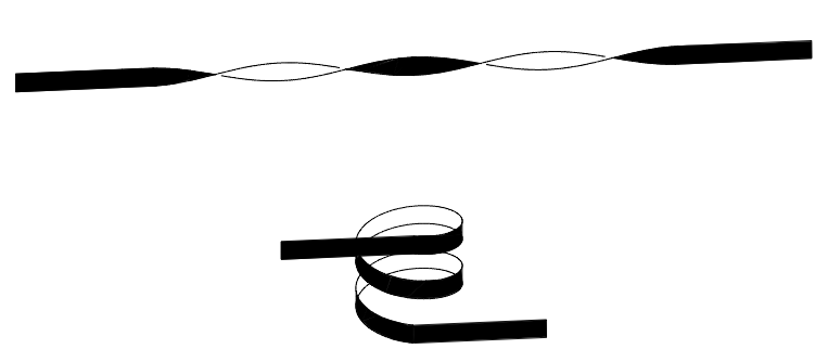
Schematic showing a closed path (extend the ends to infinity) with Linking Number \(Lk=-2\). The top image has \(Tw=-2\) and \(Wr=0\), and the bottom image has \(Tw=0\) and \(Wr=-2\).

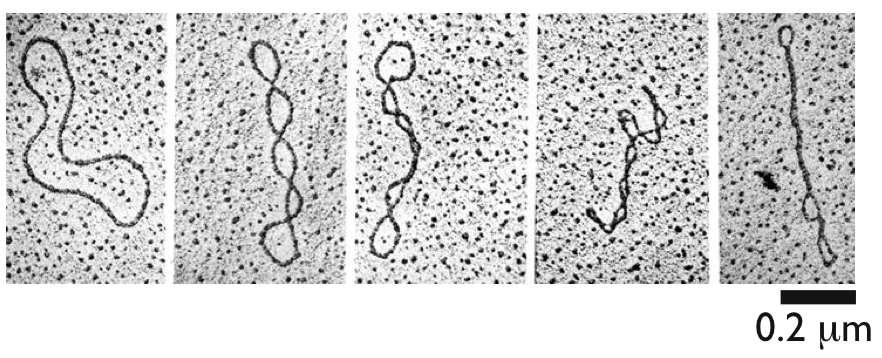
Electron micrographs of DNA with increasing values of Linking Number (see www.imsb.au.dk/~raybrown)

Models for the deformation energy

The elastic deformation energy \(E_{elas}\) must be invariant to translation and rotation of the chain. If the energy function is only dependent on the local deformation of the chain, the elastic deformation energy can be written in terms of \(\gamma\) and \(\vec{\omega}\). To lowest order, the deformation energy can generally be written

\[E_{elas} = \frac{1}{2} \int_{0}^{L} \! \! ds \left( \Omega_{i} - \Omega_{i}^{(0)} \right) A_{ij} \left( \Omega_{j} - \Omega_{j}^{(0)} \right),\]

where \(\vec{\Omega}=(\vec{\omega},\gamma)\) is the deformation 4-vector, and \(\vec{\Omega}^{(0)}\) defines the equilibrium (minimum energy) shape of the chain. The modulus tensor \(A_{ij}\) must have four positive eigenvalues for the minimum-energy shape to be stable to fluctuations. The Gaussian Chain model in 3-D [Doi1988] has a deformation energy

\[E_{elas} = \frac{3 k_{B}T}{2 b} \int_{0}^{L} \! \! ds \gamma^{2} = \frac{3 k_{B}T}{2 b^{2}} \int_{0}^{N} \! \! dn \left( \frac{\partial \vec{r}}{\partial n} \right)^{\! 2}\]

where \(n=s/b\) and \(N=L/b\).

The Wormlike Chain model in 3-D [Kratky1949] has a deformation energy

\[\beta E_{elas} = \frac{l_{p}}{2} \int_{0}^{L} \! \! ds \left( \omega_{1}^{2}+\omega_{2}^{2} \right) = \frac{l_{p}}{2} \int_{0}^{L} \! \! ds \left( \frac{\partial \vec{u}}{\partial s} \right)^{\! 2}\]

along with the inextensibility constraint \(\gamma(s) = \left| \frac{\partial \vec{r}}{\partial s} \right| = 1\) for all \(s\), and \(\beta=\frac{1}{k_{B}T}\). The persistence length \(l_{p}\) gives the bending modulus of the chain (to be discussed further in coming chapters).

The Helical Wormlike Chain model [Yamakawa1997] has a deformation energy

\[\beta E_{elas} = \int_{0}^{L} \! \! ds \left\{ \frac{A}{2} \left[ \left( \omega_{1} - \kappa \right)^{2}+ \omega_{2}^{2} \right]+ \frac{C}{2} \left( \omega_{3} - \tau \right)^{2} \right\}\]

along with the inextensibility constraint \(\gamma(s) = \left| \frac{\partial \vec{r}}{\partial s} \right| = 1\) for all \(s\), \(A\) is the bending modulus, and \(C\) is the twisting modulus. The minimum-energy shape is a helix with radius

\[a = \frac{\kappa}{\kappa^{2} + \tau^{2}}\]

and height per turn

\[h = \frac{2 \pi \tau}{\kappa^{2} + \tau^{2}}.\]

Wormlike Ribbons: Chain Statistics and Averages

We now consider a model for a wormlike ribbon, which has a straight equilibrium conformation but has distinct rigidities. The deformation energy is then given by

\[\beta E_{elas} = \int_{0}^{L} \! \! ds \left[ \frac{A_{1}}{2} \omega_{1}^{2} + \frac{A_{2}}{2} \omega_{2}^{2} + \frac{A_{3}}{2} \omega_{3}^{2} \right]\]

Following [Yamakawa1997], we define the Lagrangian density for this action as \(\mathcal{L} = \frac{A_{1}}{2} \omega_{1}^{2}+\frac{A_{2}}{2} \omega_{2}^{2}+\frac{A_{3}}{2} \omega_{3}^{2}\). We then determine the momenta \(p_{i}\) in the body-fixed frame \(\vec{t}_{i}\), such that

\[p_{i} = \frac{\partial \mathcal{L}}{\partial \omega_{i}} = A_{i} \omega_{i}\]

We then find the Hamiltonian as the Legendre transform from the Lagrangian to be

\[\begin{split}\mathcal{H} & = & \sum_{i=1}^{3} p_{i} \omega_{i} - \mathcal{L} \nonumber \\ & = & \sum_{i=1}^{3} \frac{1}{2 A_{i}} p_{i}^{2} \nonumber \\ & = & \frac{1}{2 A_{2}} \vec{p}^{2} - \frac{\Delta_{12}}{2 A_{2}} p_{1}^{2} - \frac{\Delta_{23}}{2 A_{2}} p_{3}^{2}\end{split}\]

where \(\Delta_{12} = 1 - A_{2}/A_{1}\) and \(\Delta_{23} = 1 - A_{2}/A_{3}\). We then convert the momenta into momentum operators based on the analogy between our problem and the quantum mechanical rigid rotor. From this, we find the Schrödinger equation to be

\[\frac{\partial G(\Omega|\Omega_{0}; N)}{\partial N} = \left[ \vec{p}^{2} - \Delta_{12} p_{1}^{2} - \Delta_{23} p_{3}^{2} \right] G(\Omega|\Omega_{0}; N)\]

where we non-dimensionalize the chain length as \(N = L / (2 A_{2})\). The angular momentum operators are given by

\[\begin{split}p_{1} & = & \sin \psi \frac{\partial}{\partial \theta} - \frac{\cos \psi}{\sin \theta} \frac{\partial}{\partial \phi} + \cot \theta \cos \psi \frac{\partial}{\partial \psi} \\ p_{2} & = & \cos \psi \frac{\partial}{\partial \theta} + \frac{\sin \psi}{\sin \theta} \frac{\partial}{\partial \phi} - \cot \theta \sin \psi \frac{\partial}{\partial \psi} \\ p_{3} & = & \frac{\partial}{\partial \psi}\end{split}\]

The Green’s function \(G(\Omega|\Omega_{0}; N)\) can generally be expanded in terms of Wigner functions \(\mathcal{D}_{l}^{mj}\). This expansion generally takes the form

\[G(\Omega|\Omega_{0}; N) = \sum_{lmj} \sum_{l_{0}m_{0}j_{0}} \mathcal{D}_{l}^{mj} (\Omega) \mathcal{D}_{l_{0}}^{m_{0}j_{0}^{*}} (\Omega_{0}) g_{l_{0}m_{0}j_{0}}^{lmj}(N)\]

We note that the angular momentum operators act on the Wigner functions as

\[\begin{split}p_{1} \mathcal{D}_{l}^{mj} & = & \frac{i}{2} c_{l}^{j} \mathcal{D}_{l}^{m(j+1)} +\frac{i}{2} c_{l}^{-j} \mathcal{D}_{l}^{m(j-1)} \\ p_{2} \mathcal{D}_{l}^{mj} & = & -\frac{1}{2} c_{l}^{j} \mathcal{D}_{l}^{m(j+1)} +\frac{1}{2} c_{l}^{-j} \mathcal{D}_{l}^{m(j-1)} \\ p_{3} \mathcal{D}_{l}^{mj} & = & i j \mathcal{D}_{l}^{mj}\end{split}\]

where \(c_{l}^{j} = \left[ (l-j)(l+j+1) \right]^{1/2}\). This leads to three contributions from the Hamiltonian operator acting on \(\mathcal{D}_{l}^{mj}\), given by

\[\begin{split}\vec{p}^{2} \mathcal{D}_{l}^{mj} & = & - l(l+1) \mathcal{D}_{l}^{mj} \\ p_{1}^{2} \mathcal{D}_{l}^{mj} & = & - \frac{1}{4} c_{l}^{j} c_{l}^{j+1} \mathcal{D}_{l}^{m(j+2)} - \frac{1}{4} \left( c_{l}^{j} c_{l}^{-(j+1)} + c_{l}^{-j} c_{l}^{j-1} \right) \mathcal{D}_{l}^{mj} - \frac{1}{4} c_{l}^{-j} c_{l}^{-(j-1)} \mathcal{D}_{l}^{m(j-2)} \\ p_{3}^{2} \mathcal{D}_{l}^{mj} & = & - j^{2} \mathcal{D}_{l}^{mj}\end{split}\]

Both the \(l\) and \(m\) indices are unperturbed by the Hamiltonian operator, so we have \(g_{l_{0}m_{0}j_{0}}^{lmj}\) satisfies the selection rule \(g_{l_{0}m_{0}j_{0}}^{lmj} \sim \delta_{mm_{0}} \delta_{ll_{0}}\).

We now evaluate the tangent-tangent correlation function as the basis for deriving the mean-square end-to-end distance. We first note that

\[\hat{\delta}_{z} \cdot \vec{t}_{3} = \sqrt{8 \pi^{2}/3} \mathcal{D}_{1}^{00}\]

leading to the expression

\[\langle \vec{t}_{3}(N) \cdot \vec{t}_{3}(0) \rangle = \langle \mathcal{D}_{1}^{00} (\Omega(N)) \mathcal{D}_{1}^{00} (\Omega(0)) \rangle = g_{100}^{100}\]

If we perform a Laplace transform from \(N\) to \(p\), the Schrödinger equation is used to evaluate this term as

\[p \hat{g}_{100}^{100} - 1 = \left( -2 + \Delta_{12} \right) g_{100}^{100}\]

which is inverse Laplace transformed from \(p\) to \(N\) to give

\[\langle \vec{t}_{3}(N) \cdot \vec{t}_{3}(0) \rangle = \exp \left[- (2 - \Delta_{12}) N \right]\]