Polymer Dynamics

Dynamics of a linear and ring flexible Gaussian chains (Rouse model)

We consider a flexible polymer chain that is subject Brownian forces [Doi1988]. Our goals is to determine specific dynamic properties of a linear and ring Gaussian chain. For example, we consider the dynamic motion of two chain segments relative to each other. We define this relative motion as the mean-square change in displacment (MSCD). In this development, we present a detailed derivation for the linear chain, and we provide the results for the ring polymer.

Schematic representation of the linear and ring Rouse model with definition of segments for MSCD calculation. The total chain length is \(N = 2 N_{s}\), and we consider two points on the chain located at \(n_{1} = N_{s} - \Delta = N/2 - \Delta\) and \(n_{2} = N_{s} + \Delta = N/2 + \Delta\).

We start by defining a discrete polymer chain with bead positions \(\vec{R}_{m}\), where \(m\) runs from 0 to \(n_{\mathrm{b}}\). Each bead is connected to their neighboring beads by Hookean springs, resulting in a potential force on the \(m\)-th bead \(\vec{F}_{V_{m}}\) that is given by

\[\begin{split}& & \vec{F}_{V_{m}}= \left\{ \begin{array}{c} \frac{3 k_{B}T}{g b^{2}} \left( \vec{R}_{m+1} - 2 \vec{R}_{m} + \vec{R}_{m-1} \right), \hspace{0.3in} m = 1,\ldots, n_{\mathrm{b}}-1 \\ \frac{3 k_{B}T}{g b^{2}} \left( \vec{R}_{1} - \vec{R}_{0} \right), \hspace{2in} m = 0 \\ -\frac{3 k_{B}T}{g b^{2}} \left( \vec{R}_{n_{\mathrm{b}}} - \vec{R}_{n_{\mathrm{b}}-1} \right), \hspace{1.65in} m = n_{\mathrm{b}}, \end{array} \right.\end{split}\]

where \(b\) is the Kuhn statistical segment length of the polymer [Doi1988], and \(g\) is the number of Kuhn lengths per bead. We set \(g = N/n_{\mathrm{b}}\), giving a total chain length of \(N\) Kuhn lengths.

The Langevin equation of motion for the \(m\)-th bead is given by

\[g \xi \frac{d\vec{R}_{m}(t)}{dt}=\vec{F}_{V_{m}} + \vec{F}_{B_{m}}\]

where the drag coefficient \(\xi\) is defined as the viscous drag per Kuhn length. We now take the limit of \(n_{\mathrm{b}} \rightarrow \infty\) for fixed chain length \(N\), resulting in a continuous-chain representation of the chain \(\vec{r}(n,t)\) where \(n\) is a path-length variable that runs from \(0\) to \(N\). The Langevin equation for the chain is given by

(1)\[\xi \frac{\partial \vec{r}(n, t)}{\partial t}= \frac{3 k_{B}T}{b^{2}} \frac{\partial^{2} \vec{r}(n, t)}{\partial n^{2}} + \vec{f}_{B}(n,t),\]

which is subject to the end conditions

\[\frac{\partial \vec{r}(n=0,t)}{\partial n} = \frac{\partial \vec{r}(n=N,t)}{\partial n} = 0.\]

The Brownian forces satisfy the fluctuation dissipation theorem

\[\langle \vec{f}_{B}(n,t)\vec{f}_{B}(n',t')\rangle = 2k_{B}T \xi \delta (n - n') \delta(t-t') \textbf{I}.\]

It is convenient to define a set of normal coordinates that effectively decouple the interactions implicit within the equation of motion (Eq. (1)). We define the normal modes

\[\begin{split}& & \phi_{p}(n)= \left\{ \begin{array}{c} \sqrt{2} \cos \left( \frac{\pi p n}{N} \right), \ \ p = 1,2,\ldots \\ 1, \ \ \ \ \ \ \ \ \ \ p = 0. \end{array} \right.\end{split}\]

These modes represent a complete basis set that satisfy the boundary conditions for \(\vec{r}(n,t)\). Orthogonality is demonstrated by noting

\[\int_{0}^{N} \! \! dn \phi_{p}(n) \phi_{p'}(n) = N \delta_{p,p'}.\]

The amplitude of the \(p\)-th mode \(\vec{X}_{p}(t)\) is given by

\[\vec{X}_{p}(t) = \frac{1}{N} \int_{0}^{N} \! \! dn \, \vec{r}(n,t) \phi_{p}(n),\]

and the inversion back to chain coordinates is written as

\[\vec{r}(n,t) = \sum_{p=0}^{\infty} \vec{X}_{p}(t) \phi_{p}(n).\]

Upon performing a transform to normal coordinates, we find the governing equation of motion

(2)\[\xi N \frac{d \vec{X}_{p}}{d t} = - k_{p} \vec{X}_{p} + \vec{f}_{B_{p}}\]

where \(k_{p} = \frac{3 \pi^{2} k_{B}T}{b^{2} N} p^{2}\). The \(p\)-mode Brownian force \(\vec{f}_{B_{p}}\) is given by

\[\vec{f}_{B_{p}} = \int_{0}^{N} \! \! dn \, \vec{f}_{B}(n,t) \phi_{p}(n)\]

and satisfies the fluctuation dissipation theorem

\[\langle \vec{f}_{B_{p}} (t) \vec{f}_{B_{p'}}(t') \rangle = 2 k_{B}T \xi N \delta_{pp'} \delta (t - t') \mathbf{I}.\]

A similar derivation for a ring polymer results in a treatment that is identical to the linear chain, but the normal modes for the ring polymer are continuous across the ends [i.e. \(\vec{r}(n=0,t) = \vec{r}(n=N,t)\)]. Specifically, the complete normal-mode set is separated into even and odd functions, respectively defined by

\[\begin{split}& & \phi_{p}^{(e)}(n)= \left\{ \begin{array}{c} \sqrt{2} \cos \left( \frac{2 p \pi n}{N} \right), \ \ p = 1,2,\ldots \\ 1, \ \ \ \ \ \ \ \ \ \ p = 0. \end{array} \right.\end{split}\]

and

\[\phi_{p}^{(o)}(n)= \sqrt{2} \sin \left( \frac{2 \pi p n}{N} \right), \ \ p = 1,2,\ldots\]

The even and odd normal modes satisfy the equation of motion defined in Eq. (2) with \(k_{p} = \frac{12 \pi^{2} k_{B}T}{b^{2} N} p^{2}\)

Mean-square displacement (MSD) for linear polymers

The mean-square displacement of a segment of the polymer chain is define a

(3)\[\mathrm{MSD} = \langle \left( \vec{r}(n, t) - \vec{r}(n, 0) \right)^{2} \rangle\]

for the nth segment of the chain with total length \(N\). We insert our normal-mode representation into Eq. (3), resulting in the expression

\[\mathrm{MSD} = \sum_{p=0}^{\infty} \sum_{p'=0}^{\infty} \langle \left( \vec{X}_{p}(t) - \vec{X}_{p}(0) \right) \cdot \left( \vec{X}_{p'}(t) - \vec{X}_{p'}(0) \right) \rangle \phi_{p}(n) \phi_{p'}(n)\]

The equation of motion (Eq. (2)) can be used to determine the correlation function \(\langle \vec{X}_{p}(t) \cdot \vec{X}_{p'}(0) \rangle\) (detailed discussion is found in Ref. [Doi1988]). This results in the expression

\[\langle \vec{X}_{p}(t) \cdot \vec{X}_{p'}(0) \rangle = 3 \frac{k_{B}T}{k_{p}} \exp \! \left( - \frac{k_{p}}{N \xi} t \right) \delta_{pp'}\]

for \(p \ge 1\) and

\[\langle \left( \vec{X}_{0}(t) - \vec{X}_{0}(0) \right)^{2} \rangle = 6 \frac{k_{B}T}{N \xi} t\]

We focus on the \(\mathrm{MSD}\) for the midpoint of a linear chain, thus \(n=N/2\). Inserting this into our definition of \(\mathrm{MSD}\) results in the expression for the MSD of the midpoint of a linear chain

\[\begin{split}\mathrm{MSD} & = & 6 \frac{k_{B}T}{\xi N} t + \sum_{p \, \mathrm{even}} 12 \frac{k_{B}T}{k_{p}} \left[ 1 - \exp \! \left( - \frac{k_{p}}{N \xi} t \right) \right] \\ & = & 6 \frac{k_{B}T}{\xi N} t + \sum_{p = 1}^{\infty} 12 \frac{k_{B}T}{k_{2p}} \left[ 1 - \exp \! \left( - \frac{k_{2p}}{N \xi} t \right) \right]\end{split}\]

Mean-squared change in distance (MSCD) for linear and ring polymers

We now consider the mean-square change in distance (MSCD) for a linear polymer chain. This quantity is defined as

(4)\[\mathrm{MSCD} = \langle \left( \Delta \vec{R}(t) - \Delta \vec{R}(0) \right)^{2} \rangle\]

where \(\Delta \vec{R}(t) = \vec{r}(N/2 + \Delta, t) - \vec{r}(N/2 - \Delta,t)\) where the total chain length is \(N = 2 N_{s}\). We insert our normal-mode representation into Eq. (4) to find

\[\mathrm{MSCD} = \sum_{p=1}^{\infty} \sum_{p'=1}^{\infty} \langle \left( \vec{X}_{p}(t) - \vec{X}_{p}(0) \right) \cdot \left( \vec{X}_{p'}(t) - \vec{X}_{p'}(0) \right) \rangle \left[ \phi_{p}(N/2 + \Delta) - \phi_{p}(N/2 - \Delta) \right] \left[ \phi_{p'}(N/2 + \Delta) - \phi_{p'}(N/2 - \Delta) \right]\]

The equation of motion (Eq. (2)) can be used to determine the correlation function \(\langle \vec{X}_{p}(t) \cdot \vec{X}_{p'}(0) \rangle\) (detailed discussion is found in Ref. [Doi1988]). This results in the expression

\[\langle \vec{X}_{p}(t) \cdot \vec{X}_{p'}(0) \rangle = 3 \frac{k_{B}T}{k_{p}} \exp \! \left( - \frac{k_{p}}{N \xi} t \right) \delta_{pp'}\]

Inserting this into our definition of \(\mathrm{MSCD}\) results in the expression for the linear chain

\[\begin{split}\mathrm{MSCD}^{\mathrm{(linear)}} & = & \sum_{p \, \mathrm{odd}} 48 \frac{k_{B}T}{k_{p}} \left[ 1 - \exp \! \left( - \frac{k_{p}}{N \xi} t \right) \right] \sin^{2} \left( \frac{\pi p \Delta}{N} \right) \\ & = & \sum_{p = 0}^{\infty} 48 \frac{k_{B}T}{k_{2p+1}} \left[ 1 - \exp \! \left( - \frac{k_{2p+1}}{N \xi} t \right) \right] \sin^{2} \left[ \frac{\pi (2p+1) \Delta}{N} \right]\end{split}\]

where \(k_{p} = \frac{3 \pi^{2} k_{B}T}{b^{2} N} p^{2}\) for the linear chain.

We follow a parallel derivation for the ring polymer. We note that only the odd set of normal modes contribute to \(\mathrm{MSCD}\) for the ring polymer. Taking similar steps as in the linear case, we arrive at the expression for the ring polymer

\[\mathrm{MSCD}^{\mathrm{(ring)}} = \sum_{p = 1}^{\infty} 48 \frac{k_{B}T}{k_{p}} \left[ 1 - \exp \! \left( - \frac{k_{p}}{N \xi} t \right) \right] \sin^{2} \left( \frac{2 \pi p \Delta}{N} \right)\]

where \(k_{p} = \frac{12 \pi^{2} k_{B}T}{b^{2} N} p^{2}\) for the ring polymer.

Functions contained with the ‘poly_dyn’ module

Polymer dynamics module - Rouse polymer, analytical results.

Notes

wlcstat.poly_dyn.draw_cells(linkages, min_y=0.05, max_y=0.95, locus_frac=0.7989601386481803, centromere_frac=0.7365684575389948, chr_size=17.474999999999998)

Render the model of homologous chromosomes with linkages.

Parameters

linkages (float array) – List of the link positions between the homologous chromosomes

wlcstat.poly_dyn.end_to_end_corr(t, D, N, num_modes=10000)

Doi and Edwards, Eq. 4.35

wlcstat.poly_dyn.generate_example_cell(mu, chr_size=17.474999999999998)

Generate the number and location of linkage between homologous chromosomes

Parameters

• mu (float) – Average number of linkages between chromosomes (Poisson distributed)

• chr_size (float) – Size of the chromosome (microns)

Returns

cell – List of linkage locations between the homologous chromosomes

Return type

float array (length selected from Poisson distribution)

wlcstat.poly_dyn.linear_mid_msd(t, b, N, D, num_modes=20000)

Calculate the MSD for the midpoint on a Rouse polymer

Parameters

• t (float array) – Time in seconds

• b (float) – Kuhn length (microns)

• N (float) – Chain length (in Kuhn lengths)

• D (float) – Diffusivity (microns ** 2 / second)

• num_modes (int) – Number of normal modes used in the calculation

Returns

msd – Calculated MSD for a Rouse polymer

Return type

float array (size len(t))

wlcstat.poly_dyn.linear_mid_msd_subpoly(t, b, N, D, alpha=1, num_modes=20000)

Calculate the MSD for the midpoint on a subdiffusive Rouse polymer

Parameters

• t (float array) – Time in seconds

• b (float) – Kuhn length (microns)

• N (float) – Chain length (in Kuhn lengths)

• D (float) – Diffusivity (microns ** 2 / second)

• alpha (float) – MSD scaling exponent

• num_modes (int) – Number of normal modes used in the calculation

Returns

msd – Calculated MSD for a Rouse polymer

Return type

float array (size len(t))

wlcstat.poly_dyn.linear_mscd(t, D, Ndel, N, b=1, num_modes=20000)

Compute mscd for two points on a linear polymer.

Parameters

• t ((M,) float, array_like) – Times at which to evaluate the MSCD

• D (float) – Diffusion coefficient, (in desired output length units). Equal to \(k_BT/\xi\) for \(\xi\) in units of “per Kuhn length”.

• Ndel (float) – Distance from the last linkage site to the measured site. This ends up being (1/2)*separation between the loci (in Kuhn lengths).

• N (float) – The full lengh of the linear polymer (in Kuhn lengths).

• b (float) – The Kuhn length (in desired length units).

• num_modes (int) – how many Rouse modes to include in the sum

Returns

mscd – result

Return type

(M,) np.array<float>

wlcstat.poly_dyn.linear_mscd_subpoly(t, D, Ndel, N, b=1, alpha=1, num_modes=20000)

Compute mscd for two points on a linear polymer.

Parameters

• t ((M,) float, array_like) – Times at which to evaluate the MSCD

• D (float) – Diffusion coefficient, (in desired output length units). Equal to \(k_BT/\xi\) for \(\xi\) in units of “per Kuhn length”.

• Ndel (float) – Distance from the last linkage site to the measured site. This ends up being (1/2)*separation between the loci (in Kuhn lengths).

• N (float) – The full lengh of the linear polymer (in Kuhn lengths).

• b (float) – The Kuhn length (in desired length units).

• alpha (float) – Subdiffusive powerlaw scaling exponent for diffusion

• num_modes (int) – how many Rouse modes to include in the sum

Returns

mscd – result

Return type

(M,) np.array<float>

wlcstat.poly_dyn.linear_msd_confine(t, D, Nmono, N, b=1, k_conf=1, num_modes=20000)

Compute msd for a Rouse polymer confined within a harmonic confining potential

Parameters

• t ((M,) float, array_like) – Times at which to evaluate the MSD

• D (float) – Diffusion coefficient, (in desired output length units). Equal to \(k_BT/\xi\) for \(\xi\) in units of “per Kuhn length”.

• Nmono (float) – Monomer position of the tagged locus (in Kuhn length).

• N (float) – The full lengh of the linear polymer (in Kuhn lengths).

• b (float) – The Kuhn length (in desired length units).

• k_conf (float) – Confinement strength

• num_modes (int) – how many Rouse modes to include in the sum

Returns

msd – result

Return type

(M,) np.array<float>

wlcstat.poly_dyn.linear_msd_confine_plateau(Nmono, N, b=1, k_conf=1, num_modes=20000)

Compute msd for a Rouse polymer confined within a harmonic confining potential

Parameters

• t ((M,) float, array_like) – Times at which to evaluate the MSD

• D (float) – Diffusion coefficient, (in desired output length units). Equal to \(k_BT/\xi\) for \(\xi\) in units of “per Kuhn length”.

• Nmono (float) – Monomer position of the tagged locus (in Kuhn length).

• N (float) – The full lengh of the linear polymer (in Kuhn lengths).

• b (float) – The Kuhn length (in desired length units).

• k_conf (float) – Confinement strength

• num_modes (int) – how many Rouse modes to include in the sum

Returns

msd – result

Return type

(M,) np.array<float>

wlcstat.poly_dyn.model_mscd(t, linkages, label_loc=3.5311602490318506, chr_size=17.474999999999998, nuc_radius=1, b=0.015, D=0.02, num_modes=10000)

Calculate the MSCD for the model of linked chromosomes

Parameters

• t (float array) – Time in seconds

• linkages (float array) – List of the link positions between the homologous chromosomes

• label_loc (float) – Location of the fluorescent label along the chromosome (microns)

• chr_size (float) – Length of the chromosome (microns)

• nuc_radius (float) – Radius of the nucleus (microns)

• b (float) – Kuhn length (microns)

• D (float) – Diffusivity (microns ** 2 / second)

• num_modes (int) – Number of normal modes used in the calculation

Returns

mscd_model – Calculated MSCD (microns ** 2) for the model with defined linkages

Return type

float array (size len(t))

wlcstat.poly_dyn.model_mscd_confine(t, linkages, label_loc=3.5311602490318506, chr_size=17.474999999999998, nuc_radius=1, k_conf=1, b=0.015, D=0.02, num_modes=10000)

Calculate the MSCD for the model of linked chromosomes

Parameters

• t (float array) – Time in seconds

• linkages (float array) – List of the link positions between the homologous chromosomes

• label_loc (float) – Location of the fluorescent label along the chromosome (microns)

• chr_size (float) – Length of the chromosome (microns)

• nuc_radius (float) – Radius of the nucleus (microns)

• k_conf (float) – Strength of confining potential

• b (float) – Kuhn length (microns)

• D (float) – Diffusivity (microns ** 2 / second)

• num_modes (int) – Number of normal modes used in the calculation

Returns

mscd_model – Calculated MSCD (microns ** 2) for the model with defined linkages

Return type

float array (size len(t))

wlcstat.poly_dyn.model_mscd_subpoly(t, linkages, label_loc=3.5311602490318506, chr_size=17.474999999999998, nuc_radius=1, b=0.015, D=0.02, alpha=1, num_modes=10000)

Calculate the MSCD for the model of linked chromosomes

Parameters

• t (float array) – Time in seconds

• linkages (float array) – List of the link positions between the homologous chromosomes

• label_loc (float) – Location of the fluorescent label along the chromosome (microns)

• chr_size (float) – Length of the chromosome (microns)

• nuc_radius (float) – Radius of the nucleus (microns)

• b (float) – Kuhn length (microns)

• D (float) – Diffusivity (microns ** 2 / second)

• num_modes (int) – Number of normal modes used in the calculation

Returns

mscd_model – Calculated MSCD (microns ** 2) for the model with defined linkages

Return type

float array (size len(t))

wlcstat.poly_dyn.model_mscd_subpoly_1d(t, linkages, label_loc=3.5311602490318506, chr_size=17.474999999999998, nuc_radius=1, b=0.015, D=0.02, alpha=1, num_modes=10000)

Calculate the MSCD for the model of linked chromosomes based on an effective 1-dimensional model

Parameters

• t (float array) – Time in seconds

• linkages (float array) – List of the link positions between the homologous chromosomes

• label_loc (float) – Location of the fluorescent label along the chromosome (microns)

• chr_size (float) – Length of the chromosome (microns)

• nuc_radius (float) – Radius of the nucleus (microns)

• b (float) – Kuhn length (microns)

• D (float) – Diffusivity (microns ** 2 / second)

• num_modes (int) – Number of normal modes used in the calculation

Returns

mscd_model – Calculated MSCD (microns ** 2) for the model with defined linkages

Return type

float array (size len(t))

wlcstat.poly_dyn.model_mscd_subpoly_simple(t, linkages, label_loc=3.5311602490318506, chr_size=17.474999999999998, nuc_radius=1, b=0.015, D=0.02, alpha=1, num_modes=10000)

Calculate the MSCD for the model of linked chromosomes using a simple power-law and plateau model

Parameters

• t (float array) – Time in seconds

• linkages (float array) – List of the link positions between the homologous chromosomes

• label_loc (float) – Location of the fluorescent label along the chromosome (microns)

• chr_size (float) – Length of the chromosome (microns)

• nuc_radius (float) – Radius of the nucleus (microns)

• b (float) – Kuhn length (microns)

• D (float) – Diffusivity (microns ** 2 / second)

• num_modes (int) – Number of normal modes used in the calculation

Returns

mscd_model – Calculated MSCD (microns ** 2) for the model with defined linkages

Return type

float array (size len(t))

wlcstat.poly_dyn.model_plateau(linkages, label_loc=3.5311602490318506, chr_size=17.474999999999998, nuc_radius=1, b=0.015)

Evaluate the plateau values in the MSCD

Parameters

• linkages (float array) – List of the link positions between the homologous chromosomes

• label_loc (float) – Location of the fluorescent label along the chromosome (microns)

• chr_size (float) – Length of the chromosome (microns)

• nuc_radius (float) – Radius of the nucleus (microns)

• b (float) – Kuhn length (microns)

Returns

mscd_plateau – Plateau value of the MSCD in the long-time asymptotic limit (microns ** 2)

Return type

float

wlcstat.poly_dyn.ring_mscd(t, D, Ndel, N, b=1, num_modes=20000)

Compute mscd for two points on a ring.

Parameters

• t ((M,) float, array_like) – Times at which to evaluate the MSCD.

• D (float) – Diffusion coefficient, (in desired output length units). Equal to \(k_BT/\xi\) for \(\xi\) in units of “per Kuhn length”.

• Ndel (float) – (1/2)*separation between the loci on loop (in Kuhn lengths)

• N (float) – full length of the loop (in Kuhn lengths)

• b (float) – The Kuhn length, in desired output length units.

• num_modes (int) – How many Rouse modes to include in the sum.

Returns

mscd – result

Return type

(M,) np.array<float>

wlcstat.poly_dyn.ring_mscd_subpoly(t, D, Ndel, N, b=1, alpha=1, num_modes=20000)

Compute mscd for two points on a ring.

Parameters

• t ((M,) float, array_like) – Times at which to evaluate the MSCD.

• D (float) – Diffusion coefficient, (in desired output length units). Equal to \(k_BT/\xi\) for \(\xi\) in units of “per Kuhn length”.

• Ndel (float) – (1/2)*separation between the loci on loop (in Kuhn lengths)

• N (float) – full length of the loop (in Kuhn lengths)

• b (float) – The Kuhn length, in desired output length units.

• alpha (float) – Subdiffusive powerlaw scaling exponent for diffusion

• num_modes (int) – How many Rouse modes to include in the sum.

Returns

mscd – result

Return type

(M,) np.array<float>

Example usage of ‘linear_mscd’ and ‘ring_mscd’

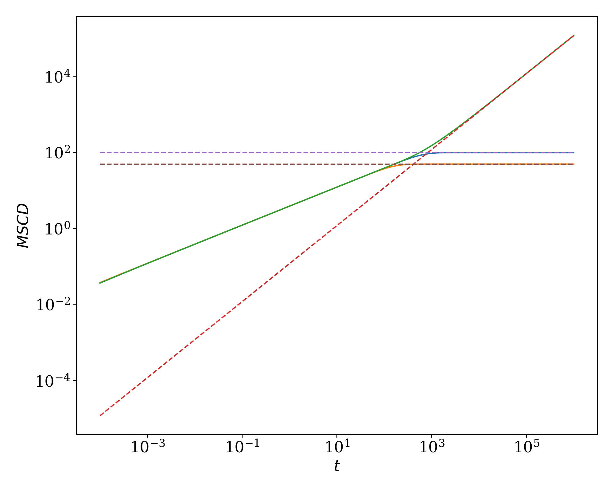
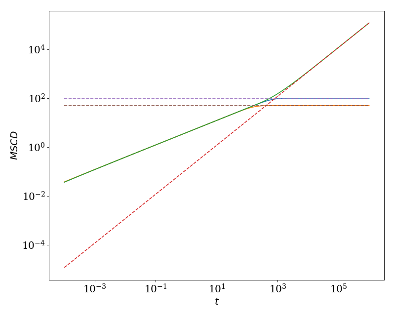
We show the solution for the MSCD for chain length \(N=100\) and \(\Delta = 25\) for both linear and ring polymers. In this plot, we also show the MSD (using ‘linear_mid_msd’) multiplied by 2, which coincides with the short-time asymptotic behavior. The long-time asymptotic behavior is found by noting

\[\mathrm{MSCD} = \langle \left( \Delta \vec{R}(t) - \Delta \vec{R}(0) \right)^{2} \rangle = \langle \Delta \vec{R}(t)^{2} \rangle - 2 \langle \Delta \vec{R}(t) \cdot \Delta \vec{R}(0) \rangle + \langle \Delta \vec{R}(0) ^{2} \rangle \rightarrow 2 \langle \Delta \vec{R}^{2} \rangle\]

which leads to the asymptotic solutions

\[\mathrm{MSCD}^{\mathrm{(linear)}} \rightarrow 4 \Delta\]

and

\[\mathrm{MSCD}^{\mathrm{(ring)}} \rightarrow \frac{2}{\frac{1}{2 \Delta} + \frac{1}{N-2 \Delta}}.\]

These asymptotic solutions are also included in the plot.

(Source code, png, hires.png, pdf)

Application of ‘linear_mscd’ and ‘ring_mscd’ to homologue pairing in meiosis

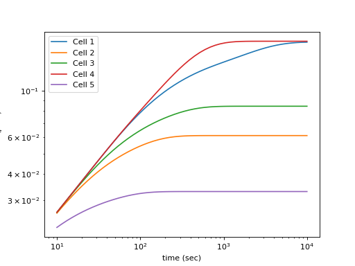
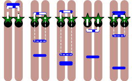
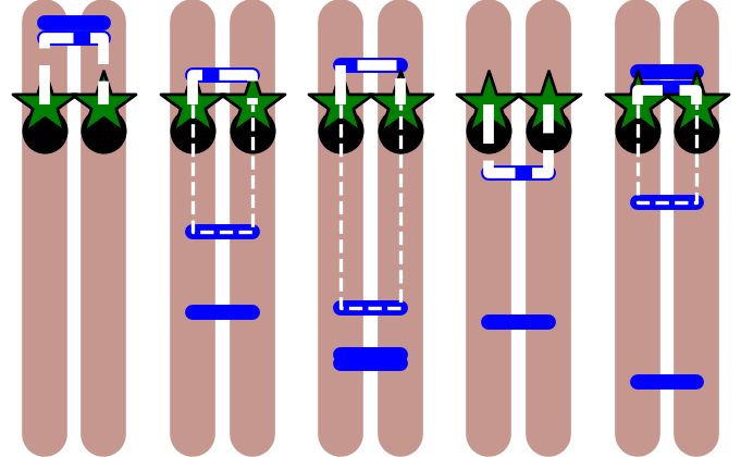
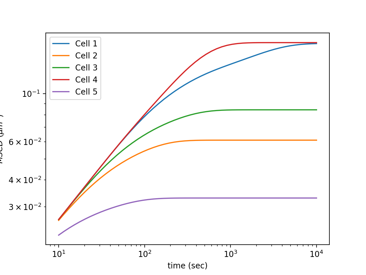
We apply ‘linear_mscd’ and ‘ring_mscd’ to the coordinated dynamics of loci on two homologous chromosomes (chromosome V in S. cerevisiae). The average number of linkages between the chromosomes is \(\mu = 4\). The length of chromosome V is approximately 577 kb, and the position of the fluorescent locus is at 177 kb. The top plot below shows the locations of the random linkages for the five example “cells”. The effective tethers holding the loci together are highlighted in white. The nearest linkage is highlighted by a thicker line. Notice that when two tethers exist, they effectively form a large chromatin loop on which the two loci live. The bottom plot shows analytical MSCDs for five different theoretical “cells”, where a Poisson-distributed number of linkages (\(\mu = 4\)) have been distributed uniformly along chr.~V, which we assume to be composed of approximately 116,000 Kuhn lengths of length.

(Source code, png, hires.png, pdf)

(png, hires.png, pdf)